Swish, mish, and serf

Swish, mish, and serf are neural net activation functions. The names are fun to say, but more importantly the functions have been shown to improve neural network performance by solving the “dying ReLU problem.” This happens when a large number of node weights become zero during training and do not contribute further to the learning process. The weights may be “trying” to be negative, but the activation function won’t allow it. The swish family of activation functions allows weights to dip negative.

Softplus can also be used as an activation function, but our interest in softplus here is as part of the definition of mish and serf. Similarly, we’re interested in the sigmoid function here because it’s used in the definition of swish.

Softplus, softmax, softsign

Numerous functions in deep learning are named “soft” this or that. The general idea is to “soften” a non-differentiable function by approximating it with a smooth function.

The plus function is defined by

x^+ =<br /> \left\{<br /> \begin{array}{ll}<br /> x & \mbox{if } x \geq 0 \\<br /> 0 & \mbox{if } x < 0 \end{array} \right.

In machine learning the plus is called ReLU (rectified linear unit) but x+ is conventional mathematical notation.

The softplus function approximates x+ by

\text{softplus}(x) = \log(1 + \exp(x))

We can add a parameter to the softplus function to control how soft it is.

\text{softplus}(x; k) = \frac{1}{k}\log\left(1 + \exp(kx)\right)

As the parameter k increases, softmax becomes “harder.” It more closely approximates x+ but at the cost of the derivative at 0 getting larger.

We won’t need other “soft” functions for the rest of the post, but I’ll mention a couple more while we’re here. Softmax is a smooth approximation to the max function

\text{softmax}(x, y) = \log\left(\exp(x) + \exp(y)\right)

and softsign is a smooth approximation to the sign function.

\text{softsign}(x) = \frac{x}{1 + |x|}

which is differentiable at the origin, despite the absolute value in the denominator. We could add a sharpness parameter k to the softmax and softsign functions like we did above.

Sigmoid

The sigmoid function, a.k.a. the logistic curve, is defined by

\sigma(x) = \frac{\exp(x)}{1 + \exp(x)} = \frac{1}{1 + \exp(-x)}

The second and third expressions are clearly equal, but I prefer to think in terms of the former, but the latter is better for numerical calculation because it won’t overflow for large x.

The sigmoid function is the derivative of the softplus function. We could define a sigmoid function with a sharpness parameter k by takind the derivative of the softplus function with sharpness parameter k.

Swish

The Swish function was defined in [1] as

\text{swish}(x) = x \, \sigma(x)

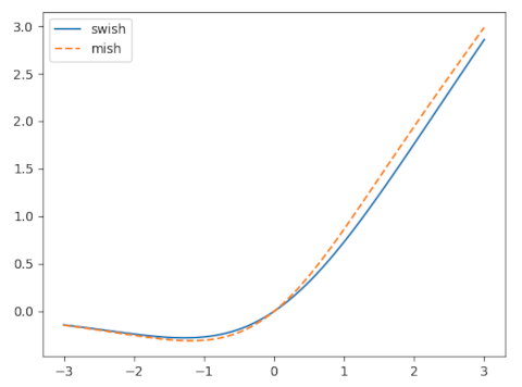
Like softplus, the Swish function is asymptotically 0 as x → −∞ and asymptotically equal to x as x → ∞. That is, for large |x|, swish(x) is approximately x+. However, unlike softplus, swish(x) is not monotone. It is negative for negative x, having a minimum around -1.278 [2]. The fact that the activation function can dip into negative territory is what addresses “the dying ReLU problem,”

Mish

The Mish function was defined in [3] as

\text{mish}(x) = x \, \tanh(\,\text{softplus}(x)\,)

The mish function has a lot in common with the swish function, but performs better, at least on the examples the author presents.

The mish function is said to be part of the swish function family, as is the serf function below.

Serf

The serf function [4] is another variation on the swish function with similar advantages.

\text{serf}(x) = x \, \text{erf}(\,\text{softplus}(x)\,)

The name “serf” comes from “log-Softplus ERror activation Function” but I’d rather pronounce it “zerf” from “x erf” at the beginning of the definition.

The serf function is hard to distinguish visually from the mish function; I left it out of the plot above to keep the plot from being cluttered. Despite the serf and mish functions being close together, the authors in [4] says the former outperforms the latter on some problems.

Numerical evaluation

The most direct implementations of the softplus function can overflow, especially when implemented in low-precision floating point such as 16-bit floats. This means that the mish and serf functions could also overflow.

For large x, exp(x) could overflow, and so computing softplus as

   log(1 + exp(x))

could overflow while the exact value would be well within the range of representable numbers. A simple way to fix this would be to have the softmax function return x when x is so large that exp(x) would overflow.

As mentioned above, the expression for the sigmoid function with exp(-x) in the denominator is better for numerical work than the version with exp(x) in the numerator.

Related posts

[1] Swish: A Self-Gated Activation Function. Prajit Ramachandran∗, Barret Zoph, Quoc V. arXiv:1710.05941v1

[2] Exact form of the minimum location and value in terms of the Lambert W function discussed in the next post.

[3] Mish: A Self Regularized Non-Monotonic Activation Function. Diganta Misra. arXiv:1908.08681v3

[4] SERF: Towards better training of deep neural networks using log-Softplus ERror activation Function. Sayan Nag, Mayukh Bhattacharyya. arXiv:2108.09598v3

Generating and inspecting an RSA private key

In principle you generate an RSA key by finding two large prime numbers, p and q, and computing n = pq. You could, for example, generate random numbers by rolling dice, then type the numbers into Mathematica to test each for primality until you find a couple prime numbers of the right size.

In practice you’d use a specialized program to find the primes and to wrap everything up in a format that software using the keys can understand. There are a lot of layers between the numbers p and q and the file that key generating software produces, and this post aims to peel back these layers a bit.

Here’s an example of generating a private key taken from The OpenSSL Cookbook.

    openssl genpkey -out fd.key -algorithm RSA \
      -pkeyopt rsa_keygen_bits:2048 -aes-128-cbc

The genpkey function can be used for generating several kinds of public keys. The option -algorithm RSA tells it that we want an RSA key, but we could have asked for an elliptic curve key. As noted in the previous post, in practice public key encryption is used to transfer symmetric encryption keys, not messages per se. The flag -aes-128-cbc tells the software the we’d like to use AES encryption with a 128-bit key in CBC (cipher block chaining) mode.

When you press enter you’ll see a flurry of dots and plus signs that show the progress of the software in generating and testing candidates for the primes p and q. Then you’ll be prompted for a password to encrypt the private key you’ve just created.

If you open the fd.key file you won’t see much:

    % cat fd.key
    -----BEGIN ENCRYPTED PRIVATE KEY-----
    MIIFLTBXBgkqhkiG9w0BBQ0wSjApBgkqhkiG9w0BBQwwHAQIdCZSKfkqh6kCAggA
    MAwGCCqGSIb3DQIJBQAwHQYJYIZIAWUDBAECBBAqbtHXkZ+uqa3rvj6qKqbRBIIE
    ...
    U6QCPcWukFyUAghHdTfjKgoAEXfOEunALoaTF6LMPsd6
    -----END ENCRYPTED PRIVATE KEY-----

This is just base 64-encoded data.

The data is encoded in two senses. It is encoded in a non-secret way, expressed in a standardized data structure, then encoded in the sense of being encrypted. The openssl command pkey will undo both levels of encoding to let us see the contents of the file.

Here’s what this produces.

    Private-Key: (2048 bit, 2 primes)
    modulus:
        00:a7:b8:39:80:0b:18:d9:db:c1:a3:c1:3a:92:89:
        ...
        7a:c5
    publicExponent: 65537 (0x10001)
    ...
    prime1:
        00:dc:8c:27:e6:7f:1c:11:d4:9c:8c:33:bf:07:57:
        ...
        97:5f:8c:4c:44:23:d2:85:f9
    prime2:
        00:c2:ae:20:80:87:da:d0:a1:66:8f:2e:90:7c:ae:
        ...
        9c:e9:8a:8b:bc:c7:71:de:2d
    ...

The exponent is the default value 65537. (More on that here.)

The large numbers are displayed in hexadecimal with colons separating pairs of hex digits. If you remove the colons and concatenate everything together, you can verify that the number called modulus is indeed the product of the numbers called prime1 and prime2. I verified this for the output above using a little Python code:

    modulus = 0xa7b839...c5
    prime1  = 0xdc8c27...f9
    prime2  = 0xc2ae20...2d
    assert(prime1*prime2 == modulus)

The file also contains four numbers that require more explanation: privateExponent, exponent1, exponent2, and coefficient. The privateExponent is described here. The remaining numbers are not strictly necessary for RSA but are used in Garner’s algorithm for more efficient decryption.

Related posts

RSA encryption in practice

At its core, RSA encryption is modular exponentiation. That is, given a message m, the encrypted form of m is

x = me mod n

where e is a publicly known exponent and n is a product of two large primes. The number n is made public but only the holder of the private key knows the factors of n, and without knowing the factors of n you can’t recover m from x, or so we assume.

You can implement RSA encryption in just a few lines of code as long as you have a way to work with very large integers.

In principle you could divide your message into segments each less than n and encrypt each segment. In practice, that would be inefficient. Instead, asymmetric (public key) cryptography is only used to exchange symmetric cryptography keys. So, for example, someone wishing to send you a long message would use RSA to share the AES key used to encrypt the rest of the transmission.

So RSA is used to transfer keys, but that’s not the whole story. As is often the case, the real world implementation of cryptography is more complicated than the mathematical core.

In 1993 RSA published its PKCS#1 standard specifying that messages should be padded a certain way. That was an improvement, but then in 1998, Daniel Bleichenbacher published what has become known as the “million message attack” against the PKCS#1 standard. There were multiple proposed fixes, but these were complicated and often implemented incorrectly.

Now the standard is RSA-OAEP (Optimal Asymmetric Encryption Padding) which combines the message with random bits before applying the RSA algorithm per se. So there’s a bit of symmetric encryption, before using asymmetric encryption to share symmetric encryption keys!

My point here is not to get into the details of the OAEP protocol, but only to point out that it’s not trivial. It is, however, secure in the sense that you can prove that if someone can break RSA-OAEP then they can break the core RSA algorithm too.

“Cryptography is a mixture of mathematics and muddle, and without the muddle the mathematics can be used against you.” — Ian Cassels

Related posts

Image above CC BY-SA 4.0 by Jm-lemmi

Code to convert words to Major system numbers

A few days ago I wrote about using the CMU Pronouncing Dictionary to search for words that decode to certain numbers in the Major mnemonic system. You can find a brief description of the Major system in that post.

As large as the CMU dictionary is, it did not contain words mapping to some three-digit numbers, so it would be good to explore a larger, or at least different, dictionary. But the CMU dictionary is apparently the largest dictionary with pronunciation openly available.

To get more pronunciation data, you’ll need to generate it. This is what linguists call the grapheme to phoneme problem. There are software packages that create phonetic spellings using large neural network models, including models trained on the CMU data.

Why quick-and-dirty is OK

However, it’s possible to do a good enough job with much simpler software. There are several reasons why we don’t need the sophistication of research software. First and foremost, we can tolerate errors. If we get a few false positives, we can skim through those and ignore them. And if we get a few false negatives, that’s OK as long as we find a few of the words we’re looking for.

Another thing in our favor is that we’re not looking for pronunciation per se, only the numbers generated from the pronunciation. The hardest part of the grapheme to phoneme problem is vowel sounds, and we don’t care about vowel sounds at all. And we don’t care about distinguishing, for example, between voiced and unvoiced variations on the th sound because they both map to 1.

Code

The Major mnemonic system is based on pronunciation, not spelling. Nevertheless, you can do a rough-and-ready conversion, adequate for our purposes, based on spelling. I take into account a minimal amount of context, such as noting that c is soft before i, e, and y, but hard before a, o, and u. The handling of ch is probably biggest source of errors because the sound of ch depends on etymology.

I wrote this as a Python script initially because I wanted to share it with someone who knows Python. But I’ll present it here in Perl because the Perl code is much more compact.

sub word2num {
    local $_ = shift;
    
    tr/A-Z/a-z/; # lower case
    
    s/ng/n/g;
    s/sch/j/g;
    s/che/k/g;
    s/[cs]h/j/g;
    s/g[iey]/j/g; # soft g -> j
    s/c[eiy]/s/g; # soft c -> s
    s/c[aou]/k/g; # hard c -> k
    s/ph/f/g;
    s/([bflmprv])\1+/\1/g; # condense double letters
    s/qu/k/g;
    s/x/ks/g;

    tr/szdnmrljgkfvpb/00123456778899/;
    tr/a-z//d; # remove remaining letters
    
    return $_
}

Perl has implicit variables, for better and for worse, and here it’s for the better. All the translation (tr//) and substitution (s//) operate in place on the implicit argument, the word sent to the function.

The corresponding Python code is more verbose:

def word2num(w):

    w = w.lower()

    w = w.replace('ng', 'n')
    w = w.replace('sch', 'j')
    w = w.replace('che', 'k')

    for x in ['gi', 'ge', 'gy', 'ch', 'sh']:
        w = w.replace(x, 'j')

    ...

The order of the replacement statements matters. For example, you want to decide whether c and g are hard before you discard the vowels.

This script works better than I expected it would for being such a dirty hack. I ran it on some large word lists looking for more alternatives to the three-digit numbers not in the output of the script processing the CMU dictionary. I list a few of the words I found here. The most amusing find was phobophobia, the fear of phobias, for 898.

Aside from filling in gaps in three-digit numbers, you could also use a script like this to search for mnemonic words in specialized lists of words, such as baseball players, or animal species, or brand names.

Software and the Allee effect

The Allee effect is named after Warder Clyde Allee who added a term to the famous logistic equation. His added term is highlighted in blue.

\frac{dN}{dt} = r N {\color{red}\left( \frac{N}{A} - 1 \right)} \left( 1 - \frac{N}{K} \right)

Here N is the population of a species over time, r is the intrinsic rate of increase, K is the carrying capacity, and A is the critical point.

If you remove Allee’s term, you get an equation saying that the rate of growth of a population is proportional to the current population size, and so growth starts out exponential, and a term (1 – N/K), which says growth slows down as the population approaches its carrying capacity.

Allee’s term (N/A – 1) says that the rate of growth becomes negative when the population falls below some threshold A. When there are too few individuals, survival becomes more difficult.

Software metaphor

I thought of the Allee effect as a metaphor for software technology after writing my previous post. In general, problems become easier to solve over time. Software development may become harder because the problems developers solve are changing, but solving old problems typically gets easier. Algorithms improve and get wrapped up for convenience. There’s something like logistic growth where tasks get easier to solve, but improvement slows down over time.

If a problem is specialized, it can run into something like the Allee effect. It becomes harder over time because fewer people are interested in it. Software isn’t maintained as fast as it degrades. Fewer people have experience with it. It’s harder to be a COBOL programmer, for example, than it used to be. But this can also apply to much more current problems. A problem that was hot five years ago can be harder to solve now than it was then, for reasons the previous post discusses.

Solved problems becoming unsolved

“That’s a solved problem. So nobody knows how to solve it anymore.”

Once a problem is deemed “solved” interest in the problem plummets. “Solved” problems may not be fully solved, but sufficiently solved that the problem is no longer fashionable. Practical issues remain, but interest moves elsewhere.

The software written for the problem slowly decays. Of course the software itself doesn’t change, but the world around the software changes, and the effect is the same. More on that here.

I spent a couple hours this morning trying to build several different software packages that supposedly fully solve a problem that was fashionable not that long ago. But it doesn’t take long for links to break, for software to accumulate breaking changes, etc.

I’ve often gotten consulting jobs to re-solve a “solved” problem. The problem had been settled for most cases, but my client was very interested in what others deemed an unimportant corner case. One man’s corner case is the center of another man’s world.

The cobbler’s son

There’s an old saying “The cobbler’s son has no shoes.” It’s generally taken to mean that we can neglect to do for ourselves something we do for other people.

I’ve been writing a few scripts for my personal use, things I’ve long intended to do but only recently got around to doing.

I said something about this and someone pointed out that what I said rhymed. With a little editing I turned this into a little couplet:

The cobbler’s son is getting some shoes:
Writing some scripts for myself to use.

I won’t be blogging about my scripts because they’re not interesting. As I commented here, really useful productivity tools are not interesting to a wide audience precisely because they’re so specialized.

Date sequence from the command line

I was looking back at Jeroen Janssen’s book Data Science at the Command Line and his dseq utility caught my eye. This utility prints out a sequence of dates relative to the current date. I’ve needed this and didn’t know it.

Suppose you have a CSV file and you need to add a column of dates as the first column. I’d probably open a spreadsheet, create a column of the dates I needed, then open the CSV file and paste in the column of dates.

With Jeroen’s utility I could run

    dseq 5 | paste -d, - foo.csv

to create the same sequence of dates and add them as the first column of the file foo.csv. The option -d, tells paste to use a comma as the field separator rather than the default tab. The dash tells paste to use the piped output from dseq as its first input file.

You can run dseq three ways. With one argument, such as the 5 above, it returns the next five days from today (starting with tomorrow). With two arguments, the first is the beginning and the second is the end. With three arguments, the middle argument is an increment. As the source file summarizes it:

    # Usage: dseq LAST
    #    or: dseq FIRST LAST
    #    or: dseq FIRST INCREMENT LAST

If you just want to use dseq, grab it here. If you’d like to understand how dseq is implemented, maybe in order to modify it, keep reading.

How it works

The code is a clever one-liner:

    seq -f "%g day" "$@" | date --file - +%F

The source file has 17 lines: a shebang, several lines of documentation, and one line of code.

The one-liner starts with seq, a builtin utility that produces a sequence of integers. Like many command line utilities, seq is trivial, but it composes nicely with other utilities. And so it can be used in a pipeline to create useful scripts, as it does above.

The argument "$@" simply passes on the arguments of the script calling seq as arguments to seq. So the arguments of dseq become the arguments to seq.

The rest of the call to seq is formatting. It tells seq to append ” day” after each number. The command

    seq -f "%g day" 5

produces

    1 day
    2 day
    3 day
    4 day
    5 day

This creates strings which the date utility will interpret.

The command

    date -d "1 day"

returns the date one day from now. It includes the time, so it’s the date and time 24 hours from now.

The command

    date -d "1 day" +%F

uses the format string +%F to format the date like YYYY-MM-DD, chopping off the time.

The date option --file says to take a file as input and process each line as if it were passed into date with the -d option. The dash option says to use standard input as the file, just as the example with the paste command above used dash to signify standard input, i.e. the output of the command to the left of the pipe symbol.

Note that this script works with the GNU coreutils implementation of date. It does not work, for example, with the version of date that ships with MacOS.

Up-down permutations

An up-down permutation of an ordered set is a permutation such that as you move from left to right the permutation alternates up and down. For example

1, 5, 3, 4, 2

is an up-down permutation of 1, 2, 3, 4, 5 because

1 < 5 > 3 < 4 > 2.

Up-down permutations are also called alternating permutations for obvious reasons. The number of up-down permutations of a set of size n is often denoted A(n) because these permutations were first studied by Désiré André. It is also sometimes denoted En, where the E alludes to Euler.

André found the generating function for A(n):

\sum_{n=0}^\infty A(n) \frac{x^n}{n!} = \sec x + \tan x.

You could read this as saying sec(x) + tan(x) is the exponential generating function for A(n) or as saying sec(x) + tan(x) is the ordinary generating function for

P(n) =\frac{A(n)}{n!}

where P(n) is the proportion of all permutations of the digits 1 through n which are alternating permutations.

It’s amazing that up-down permutations have anything to do with trig functions, but they do.

Knowing the (exponential) generating function for A(n) lets us use generating function techniques to prove various things about these number. For example, we can use the generating function to discover their asymptotic behavior.

The secant and tangent functions are well behaved at 0, but both have a singularity at π/2. This means the generating function above is not just a formal power series but an analytic power series with radius of convergence π/2, the distance from the center of the power series to the closest singularity. It follows that

P(n) = {\cal O}\left( \left( \frac{2}{\pi} \right)^n \right)

and so the proportion of permutations which are alternating permutations decreases exponentially for large n.

Related posts

Variance of binned data

Suppose you have data that for some reason has been summarized into bins of width h. You don’t have the original data, only the number of counts in each bin.

You can’t exactly find the sample mean or sample variance of the data because you don’t actually have the data. But what’s the best you can do? A sensible approach would be to imagine that the contents of each bin represents samples that fell in the middle of the bin. For example, suppose your data were rounded down to the nearest integer. If you have 3 observations in the bin [5, 6] you could think of that as the value 5.5 repeated three times.

When we do this, we don’t recover the data set, but we create a pseudo data set that we can then find the sample mean and sample variance of.

This works well for estimating the mean, but it overestimates the variance. William Sheppard (1863–1936) recommended what is now known as Sheppard’s correction, subtracting h²/12 from the sample variance of the pseudo data. Richardson’s paper mentioned in the previous post fits Sheppard’s correction into the general framework of “the deferred approach to the limit.”

A more probabilistic justification of Sheppard’s correction is that h²/12 is the variance of a uniform random variable over an interval of width h. You could think of Sheppard’s correction as jittering the observations uniformly within each bin.

Let’s do a little simulation to demonstrate the accuracy of estimating the sample variance with and without Sheppard’s correction.

    from numpy import random, floor
    from scipy.stats import norm

    random.seed(20230731)

    numruns = 1000
    rawbias = 0
    sheppardbias = 0
    for run in range(numruns):
        y = norm(0, 3).rvs(size=1000)
        ypseudo = floor(y) + 0.5
        v = ypseudo.var(ddof=1)
        rawbias += abs(v - y.var(ddof=1))
        sheppardbias += abs(v - y.var(ddof=1) - 1/12)

    print(rawbias/numruns, sheppardbias/numruns)

This Python script computes the variance of the pseudodata, with and without the Sheppard correction, and compares this value to the sample variance of the actual data. This process is repeated one thousand times.

On average, the uncorrected variance of the pseudodata was off by 0.0875 compared to the variance of the actual data. With Sheppard’s correction this drops to an average of 0.0442, i.e. the calculation with Sheppard’s correction was about 2 times more accurate.