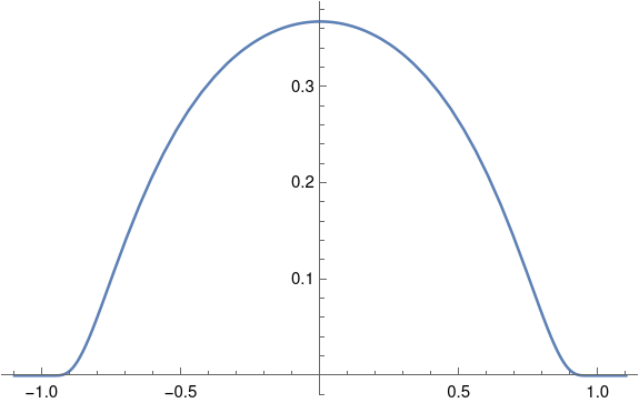
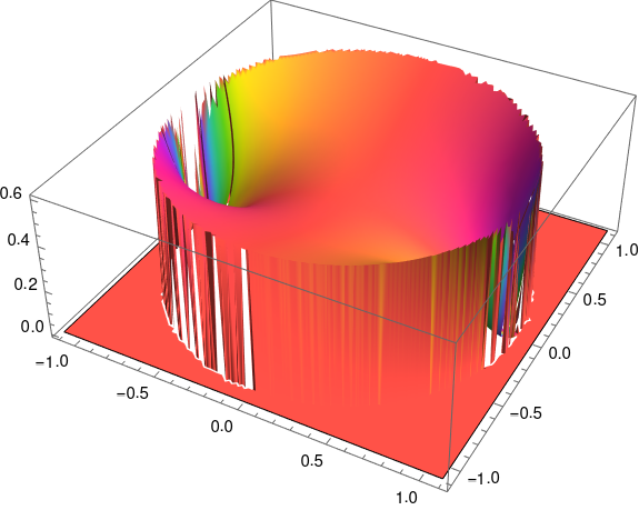
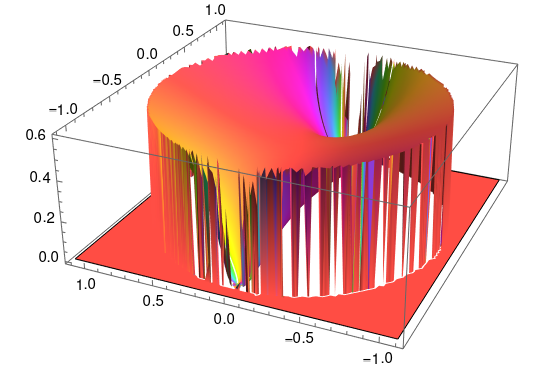
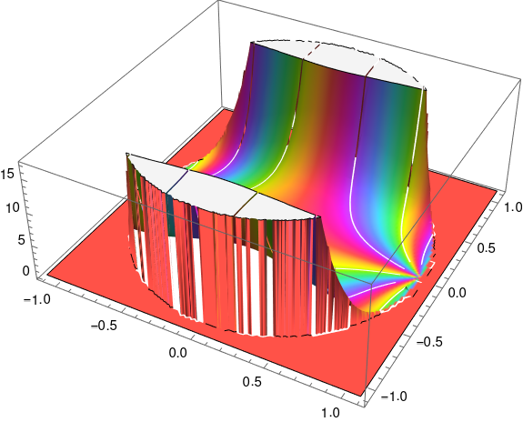
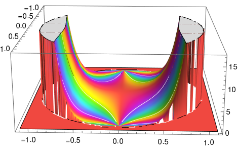
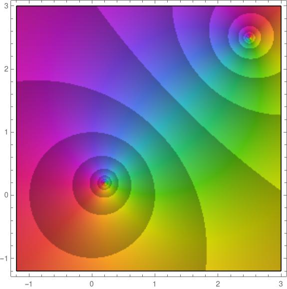
The previous post concerned the function
h(z) = exp(-1/(1 – z² )).
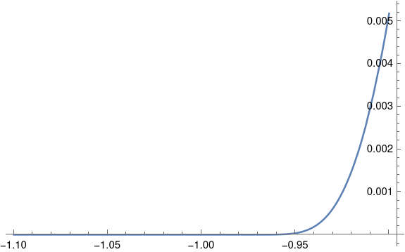
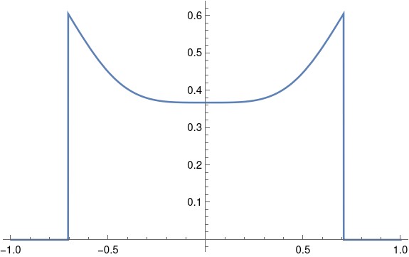
We said that the function is badly behaved near -1 and 1. How badly?
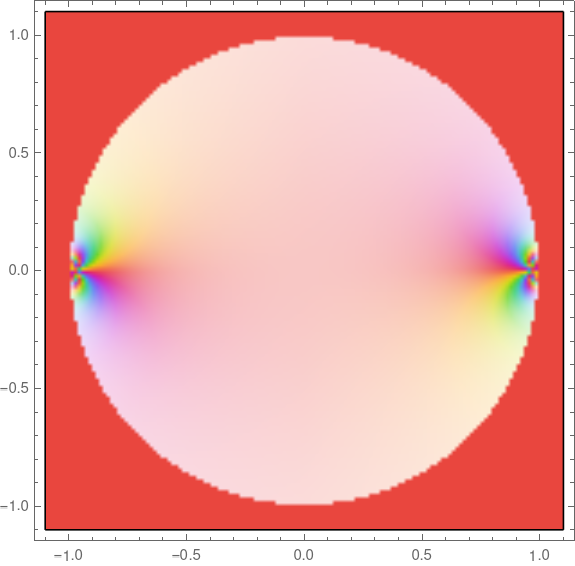
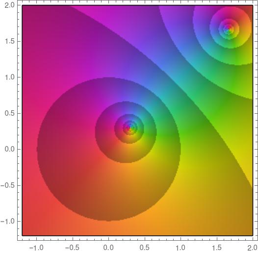
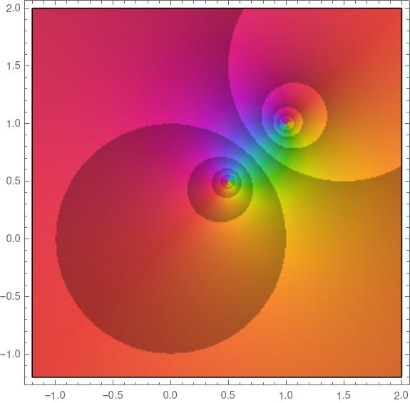
The function has essential singularities at -1 and 1. This means that not only does h blow up near these points, it blows up spectacularly.
Picard’s theorem says that if a meromorphic function f has an essential singularity at z0, then near z0 the function takes on every value in the complex plane infinitely often. That’s almost true: Picard’s theorem says f can miss one point.
Suppose we take a little disk around 1 and a complex number w. Then Picard’s theorem says that there are infinitely many solutions to the equation
h(z) = w
inside the disk, except possibly for one value of w. Since the exponential function is never 0, we know that 0 is the one value h cannot take on. So for any non-zero w, we can find an infinite number of solutions to the equation above.
OK, so let’s actually do it. Let’s pick a w and look for solutions. Today’s June 24, so let’s pick w = 6 + 24i. We want to find solutions to
exp(-1/(1 – z²)) = 6 + 24i.
Taking the log of both sides, we need to find values of z such that
-1/(1 – z²) = log(6 + 24i)
This step should make you anxious. You can’t just take logarithms of complex numbers willy nilly. Which value of the logarithm do you mean? If we pick the wrong logarithm values, will we still get solutions to our equation?
Let’s back up and say what we mean by a logarithm of a complex number. For a non-zero complex number z, a logarithm of z is a number w such that exp(w) = z. Now if z is real, there is one real solution w, hence we can say the logarithm in the context of real analysis. But since
exp(w + 2πin) = exp(w)
for any integer n, we can add a multiple of 2πi to any complex logarithm value to get another.
Now let’s go back and pick a particular logarithm of 6 + 24i. We’ll use the “principal branch” of the logarithm, the single-valued function that extends the real logarithm with a branch cut along the negative real axis. This branch is often denoted Log with a capital L. We have
Log(6 + 24i) = 3.20837 + 1.32582i.
When we take the logarithm of both sides of the equation
exp(-1/(1 – z²)) = 6 + 24i.
we get an infinite sequence of values on both sides:
2πin – 1/(1 – z²) = 2πim + Log(6 + 24i)
for integers n and m. For each fixed value of n and m the equation above is a quadratic equation in z and so we can solve it for z.
Just to make an arbitrary choice, set n = 20 and m = 22. We can then ask Mathematica to take solve for z.
NSolve[40 Pi I - 1/(1 - z^2) == 44 Pi I Log[6 + 24 I], z]
This gives two solutions:
z = -0.99932 + 0.00118143i
and
z = 0.99932 – 0.00118143i.
In hindsight, of course one root is the negative of the other, because h is an even function.
Now we don’t need n and m in
2πin – 1/(1 – z²) = 2πim + Log(6 + 24i)
because we can consolidate the move 2πim to the left side and call n – m the new n. Or to put it another way, we might as well let m = 0.
So our solutions all have the form
2πin – Log(6 + 24i) = 1/(1 – z²)
z² = 1 + 1/(Log(6 + 24i) – 2πin).
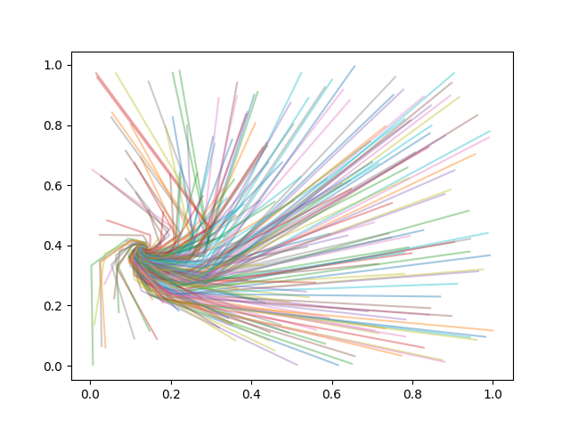
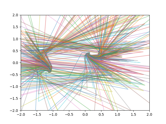
The larger n gets, the closer z gets to 1. So this shows constructive what Picard said would happen: we have a sequence of solutions converging to 1, so no matter how small a neighborhood we take around 1, we have infinitely many solutions in that neighborhood, i.e. h(z) = 6 + 24i infinitely often.