Inversion in the unit circle is a way of turning the circle inside-out. Everything that was inside the circle goes outside the circle, and everything that was outside the circle comes in.
Not only is the disk turned inside-out, the same thing happens along each ray going out from the origin. Points on that ray that are inside the circle go outside and vice versa. In polar coordinates, the point (r, θ) goes to (1/r, θ).
Complex numbers
In terms of complex numbers, inversion in the unit circle amounts to taking the reciprocal and the conjugate (in either order, because these operations commute). This is the same as dividing a complex number by the square of its magnitude. Proof:
![]()
There are two ways to deal with the case z = 0. One is to exclude it, and the other is to say that it maps to the point at infinity. This can be made rigorous by working on the Riemann sphere rather than the complex plane. More on that here.
Inverting a hyperbola
The other day Alex Kantorovich pointed out on Twitter that “the perfect figure 8 (or infinity) is simply the inversion through a circle of a hyperbola.” We’ll demonstrate this with Mathematica.
What happens to a point on the hyperbola
![]()
when you invert it through a circle? If we think of x and y as the real and imaginary parts of a complex number, the discussion above shows that the point (x, y) goes to the same point divided by its length squared.
![]()
Let (u, v) be the image of the point (x, y).

Then we have
![]()
and
![]()
because x² − y² = 1. Notice that the latter is the square of the former, i.e.
![]()
Now we have everything to make our plot. The code
ContourPlot[{
    x^2 + y^2 == 1,
    x^2 - y^2 == 1,
    x^2 - y^2 == (x^2 + y^2)^2},
    {x, -3, 3}, {y, -3, 3}]
produces the following plot.
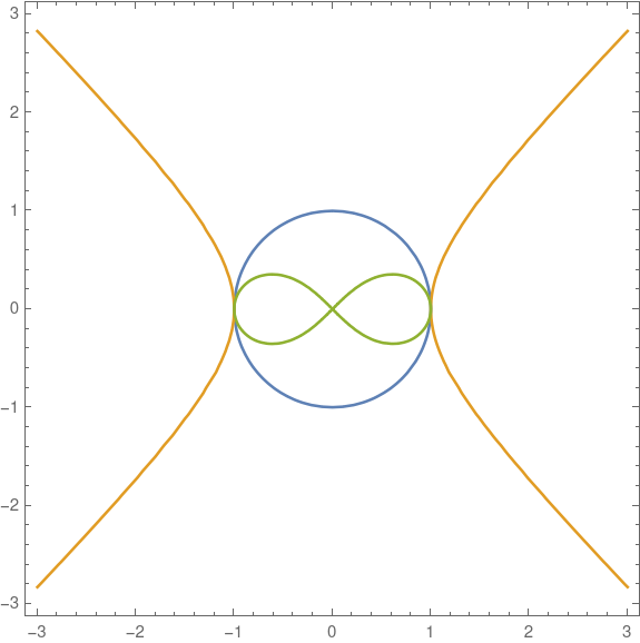
The blue circle is the first contour, the orange hyperbola is the second contour, and the green figure eight is the third contour.