The motion of a falling body of mass m is given by

where the term −kvr accounts for drag due to air resistance. One can derive r = 2 under simple physical assumptions, but if I remember correctly other values of r may be more realistic in certain circumstances. I don’t know much about the physics here; if you know about the use of other values of r, please let me know by leaving a comment.
Terminal velocity
When r = 1 or r = 2 the differential equation above can be solved in terms of elementary functions, but otherwise it cannot. Nevertheless one can show that for all values of r the object reaches a terminal velocity, and calculate that velocity without explicitly solving the differential equation. William Waterhouse demonstrated this in a one-page article [1]. He rewrites the equation to look at time as a function of velocity rather than velocity as a function of time

and concludes

He notes that the integral diverges as v approaches

and so that is the terminal velocity, i.e. it takes an infinite amount of time to achieve this velocity. Waterhouse recommends this derivation as “a good example of deriving information about a problem without knowing an explicit solution.”
I would add that such an approach is the norm, not an exception. A closed-form solution to a differential equation in nice when you can get it, but usually not possible. And even when you can find a closed-form solution, you may be able to achieve your goal more directly by not using it.
Hypergeometric solution
I suspected the differential equation could be solved for general values of r using special functions, and that is the case. Mathematica was able to evaluate the integral for t as a function of v in terms of a hypergeometric function.

When I asked Mathematica to solve the differential equation directly, it said that the solution is the inverse function of the function above. Apparently Waterhouse and Mathematica agree that it is easier to think of t as a function of v rather than the original formulation.
The notation 2F1 indicates there are two upper parameters and one lower parameter. In our application, the upper parameters are 1 and 1/r, the lower parameter is 1 + 1/r, and the function is evaluated at gkvr/m. You can find a brief introduction to hypergeometric functions here. A hypergeometric function 2F1 has a singularity at 1, and so we could derive the terminal velocity from the explicit solution.
Mathematica implementation
Let c = gk/m. Then we can express velocity as a function of time in Mathematica by
    f[r_, c_, v_] := InverseFunction
    [
        #1 Hypergeometric2F1[1, 1/r, 1 + 1/r, c #1^r] &
    ][t]
and use this to make plots of the velocity for various values of c and r.
The following sets c = 2 and varies r over 1, 1.1, 1.2, … 2.
Plot[Table[f[2, d/10, t], {d, 10, 20}], {t, 0, 4}, PlotRange -> All]
Here’s the output.
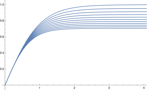
The terminal velocity decreases as r increases. The opposite is true for c < 1.
[1] William C. Waterhouse. A Fact about Falling Bodies. Mathematics Magazine, Vol. 44, No. 1 (Jan., 1971), pp. 33–34. The article straddles two pages, but takes up less than half of each page.

![\begin{align*} \text{I} \hspace{1cm} & (1+x)^{m_1} (1-x)^{m_2} \,\,[-1 \leq x \leq 1] \\ \text{II} \hspace{1cm} & (1 - x^2)^m \,\, [ -1 \leq x \leq 1] \\ \text{III} \hspace{1cm} & x^m \exp(-x) \,\, [0 \leq x] \\ \text{IV} \hspace{1cm} & (1 + x^2)^{-m} \exp(-v \arctan x) \\ \text{V} \hspace{1cm} & x^{-m} \exp(-1/x) \,\, [0 \leq x] \\ \text{VI} \hspace{1cm} & x^{m_2}(1 + x)^{-m_1} \,\,[0 \leq x] \\ \text{VII} \hspace{1cm} & (1 + x^2)^{-m}\\ \text{VIII} \hspace{1cm} & (1 + x)^{-m} \,\, [0 \leq x \leq 1] \\ \text{IX} \hspace{1cm} & (1 + x)^{m} \,\, [0 \leq x \leq 1] \\ \text{X} \hspace{1cm} & \exp(-x) \,\, [0 \leq x] \\ \text{XI} \hspace{1cm} & x^{-m} \,\,[1 \leq x] \\ \text{XII} \hspace{1cm} & \left( (g+x)(g-x)\right)^h \,\, [-g \leq x \leq g] \end{align*}](https://www.johndcook.com/pearson_distributions.svg)