Eliminating terms from higher-order differential equations

Posted on 19 November 2022 by John

This post ties together two earlier posts: the previous post on a change of variable to remove a term from a polynomial, and an older post on a change of variable to remove a term from a differential equation. These are different applications of the same idea.

A linear differential equation can be viewed as a polynomial in the differential operator D applied to the function we’re solving for. More on this idea here. So it makes sense that a technique analogous to the technique used for “depressing” a polynomial could work similarly for differential equations.

In the differential equation post mentioned above, we started with the equation

and reduced it to

using the change of variable

$u(x) = \exp\left( \frac{1}{2} \int^x p(t)\,dt\right ) y(x)$

So where did this change of variables come from? How might we generalize it to higher-order differential equations?

In the post on depressing a polynomial, we started with a polynomial

$p(x) = ax^n + bx^{n-1} + cx^{n-2} + \cdots$

and use the change of variables

$x = t - \frac{b}{na}$

to eliminate the xⁿ⁻¹ term. Let’s do something analogous for differential equations.

Let P be an nth degree polynomial and consider the differential equation

We can turn this into a differential

where the polynomial

$Q(D) = P\left(D - \frac{p}{n}\right)$

has no term involving Dⁿ⁻¹ by solving

$\left(D - \frac{p}{n}\right) u = D y$

which leads to

$u(x) = \exp\left( \frac{1}{n} \int^x p(t)\,dt\right ) y(x)$

generalizing the result above for second order ODEs.

Elliptic coordinates and Laplace’s equation

Posted on 9 November 2022 by John

In rectangular coordinates, constant values of x are vertical lines and constant values of y are horizontal lines. In polar coordinates, constant values of r are circles and constant values of θ are lines from the origin.

In elliptic coordinates, the position of a point is specified by two numbers, μ and ν. Constant values of μ are ellipses and constant values of ν are hyperbolas. (Elliptic coordinates could just as easily have been called hyperbolic coordinates, but in applications we’re usually more interested in the ellipses and so the conventional name makes sense.)

As with rectangular and polar coordinates, elliptic coordinates are orthogonal, i.e. holding each coordinate constant separately gives two curves that are perpendicular where they intersect.

Here’s a plot, with curves of constant μ in blue and curves of constant ν in green.

Graph paper for elliptic coordinates

The correspondence between rectangular and elliptic coordinates is given below.

x = a cosh μ cos ν
y = a sinh μ sin ν

The value of a can be chosen for convenience. More on that below.

Notice that elliptic coordinates area approximately polar coordinates when μ is large. This is because cosh(μ) approaches sinh(μ) as μ increases. For small values of μ elliptic coordinates are very different from polar coordinates.

The purpose of various coordinate systems is to adapt your coordinates to the structure of your problem. If you’re working with something that’s radially symmetric, polar coordinates are natural. And if you’re working with an ellipse, say you’re computing the electric field of an ellipse with uniform charge, then elliptic coordinates are natural. Ellipses can be described by one number, the value of μ.

Separation of variables

However, the real reason for specialized coordinate systems is solving partial differential equations. (Differential equations provided the motivation for a great deal of mathematics; this is practically an open secret.)

When you first see differential equations, the first, and possibly only, technique for solving PDEs you see is separation of variables. If you have PDE for a function of two variables u(x, y), you first assume u is the product of a function of x alone and a function of y alone:

u(x, y) = X(x) Y(y).

Then you stick this expression into your PDE and get independent ODEs for X and Y. Then sums of the solutions (i.e. Fourier series) solve your PDE.

Now, here’s the kicker. We could do the same thing in elliptic coordinates, starting from the assumption

u(μ, ν) = M(μ) N(ν)

and stick this into our PDE written in elliptic coordinates. The form of a PDE changes when you change coordinates. For example, see this post on the Laplacian in various coordinate systems. When you leave rectangular coordinates, the Laplacian is no longer simply the sum of the second partials with respect to each variable. However, separation of variables still works for Laplace’s equation using elliptic coordinates.

Separable coordinate systems get their name from the fact that the separation of variables trick works in that coordinate system. Not for all possible PDEs, but for common PDEs like Laplace’s equation. Elliptic coordinates are separable.

If you’re solving Laplace’s equation on an ellipse, say with a constant boundary condition, the form of the solution is going to be complicated in rectangular coordinates, but simpler in elliptic coordinates.

Confocal elliptic coordinates

The coordinate ellipses, curves with μ constant, are ellipses with foci at ±a; you can choose a so that a particular ellipse you’re interested has a particular μ value, such as 1. Since all these ellipses have the same foci, we say they’re confocal. But confocal elliptic coordinates are something slightly different.

Elliptic coordinates and confocal elliptic coordinates share the same coordinate curves, but they label them differently. Confocal elliptic coordinates (σ, τ) are related to (ordinary) elliptic coordinates via

σ = cosh μ
τ = cos ν

Laplace’s equation is still separable under this alternate coordinate system, but it looks different; the expression for the Laplacian changes because we’ve changed coordinates.

Trading generalized derivatives for classical ones

Posted on 18 October 2022 by John

Generalized functions have generalized derivatives. This is how we make sense of things like delta “functions” that are not functions, or functions that are not differentiable satisfying a differential equation. More on that here.

A major theme in the modern approach to partial differential equations is to first look for solutions in a space of generalized functions, then (hopefully) prove that the generalized function that solves your equation is a plain old function with derivatives in the classical sense.

You can differentiate generalized functions as many times as you’d like; the derivatives always exist, but these derivatives may not correspond to ordinary functions, i.e. may not be regular distributions [1]. And if the (generalized) derivatives are regular distributions, the functions they correspond to may not have as many (classical) derivatives as you’d like.

Rather than generalized derivatives existing, we’re primarily interested in generalized derivatives being regular and having finite Lebesgue norms. If generalized functions are “nice” in this sense, then we can “trade” them for classical functions, and the Sobolev embedding theorem sets the “exchange rate” for the trade.

There are a lot of variations on the Sobolev embedding theorem, but one version of the theorem, but one version says that if a function f on ℝⁿ has generalized derivatives up to order k that all correspond to L^p functions, then f is equal (almost everywhere) to a function that has r derivatives, with each of the derivatives being Hölder continuous with exponent α if

n < p

and

r + α < k − n/p.

[1] A distribution is a continuous linear functional on a space of test functions. If the effect of a distribution on a test function φ is equal to the integral of the product of a function f and φ, then the distribution is called regular, and we leave the distinction between the distribution and the function f implicit.

The Dirac delta function δ acts on a test function φ by returning φ(0). This is not a regular distribution because there is no function you can integrate against φ and always get φ(0) out.

A more direct approach to series solutions

Posted on 12 October 2022 by John

In the previous post we found a solution to

using operator calculus, i.e. treating the differential operator D like a number and doing tricks with it. See the earlier post for a justification of why we can get away with unorthodox manipulations.

We can generalize the method of the previous post to say that a solution to any differential equation of the form

is given by

$y = \frac{1}{p(D)} f(x).$

In the previous post we had

and

but the method works more generally.

We then find a power series for 1/p(D), most likely by partial fraction decomposition, and apply the result to f(x). There may be a fair amount of labor left, but it’s purely calculus; all the differential equation work is done.

Conceptually, this method subsumes other differential equation techniques such as undetermined coefficients and power series solutions.

Let’s use this method to find an approximate solution to

$y'' + 7y' + 12 = \zeta(x)$

where ζ(x) is the Riemann zeta function.

In the previous post we worked out that

$\frac{1}{D^2 + 7D + 12} = \frac{1}{D+3} - \frac{1}{D+4} = \frac{1}{12} - \frac{7}{144}D + \frac{37}{1728}D^2 + {\cal O}(D^3)$

and so an approximate solution to our differential equation near 0 is

$y(x) = \frac{1}{12}\zeta(0) - \frac{7}{144} \zeta'(0) + \frac{37}{1728}\zeta''(0) + {\cal O}(x^3).$

Numerically this works out to

If you want more terms, carry the series for 1/(D² + 7D + 12) out to more terms.

Operator calculus

Posted on 12 October 2022 by John

Students who take a course in differential equations don’t really learn how to solve differential equations. The problems whose solutions they reproduce were solved over 300 years ago. The methods taught in undergraduate ODE classes are in some sense mnemonics, a way to remember a solution discovered long ago.

Abandon hope of originality

The more scrupulous students in an ODE class cringe at being told “Guess a solution of the form …” because it seems like cheating. They may think “But I really want to learn how to solve things on my own.” This objection isn’t often addressed in part because it’s not often said out loud. But if it were explicitly stated, here’s one way to answer it.

That’s great that you want to learn how to solve differential equations on your own. But solving differential equations, in the sense of finding closed-form solutions by hand, is really hard, and unlikely to succeed. The differential equations that come up in application, that have closed-form solutions, and whose solutions can be calculated by hand in under an hour have been known since the Bernoulli’s. If this is an exaggeration, it’s a slight exaggeration.

You will learn some useful things in this class, and you may even get your first exposure to ideas that latter lead you to do original mathematics [1]. But if so, that original mathematics probably won’t be finding new closed-form solutions to useful differential equations.

This changes the perspective of the ODE class. Instead of pretending that students are going to learn how to solve differential equations ex nihilo, we can be honest that students are going to learn how to “look up” solutions to solved problems. Learning how to look up these solutions is not trivial, and in fact it takes about a semester to learn. You can’t literally look up the solution to a particular differential equation in all its specifics, but you can learn to follow the recipes for classes of equations

The role of rigor

There is a time for everything under the sun. A time for rigor and a time for handwaving. A time to embrace epsilons and a time to shun epsilons.

You can learn a lot of important reusable analysis techniques in the context of differential equations. And if that’s the goal, being rigorous is good. But if the goal is to recall the solution to a solved problem, then it’s expedient to use dirty hacks; think of them almost as mnemonics rather than as solution techniques.

Once you have a candidate solution in hand, you can always rigorously verify that it works by sticking it into the differential equation. In that sense you’re not sacrificing rigor at all.

Operator calculus

Operator calculus treats the differential operator D as a formal symbol and does calculus with it as if it were a number. This is commonly called an abuse of notation, but it has a certain elegance to it. The manipulations could be made rigorous, though not by students in an undergraduate ODE class.

Operator calculus is very powerful, and with great power comes great responsibility. It is not often taught to undergraduates, and for good reason. Sometimes formal operations are justified and sometimes they’re not. Misuse can lead to results that are simply wrong and not just illegally obtained. With that said, let’s jump in.

Let’s find a solution [2] to

Writing the differential operator as D the equation becomes

and so the solution is obviously (!)

$y = \frac{1}{D^2 + 7D + 12} x^2.$

“You can’t just divide by a differential operator like that!” Oh yeah? We’re going to do more than that. We’re going to break it into partial fractions and power series!

$\frac{1}{D^2 + 7D + 12} = \frac{1}{D+3} - \frac{1}{D+4} = \frac{1}{12} - \frac{7}{144}D + \frac{37}{1728}D^2 + {\cal O}(D^3)$

The last term means terms involving D³ and higher powers of D.

Now the first derivative of x² is 2x, the second derivative is 2, and all higher derivatives are 0. So when we apply the operator series above to x² only the terms up to D² contribute anything. From this we can tell that

$\frac{1}{12}x^2 - \frac{7}{72}x + \frac{37}{864}$

is a solution to our differential equation. You may be deeply skeptical of how we got here, and good for you if you are, but it’s easy to show that this is in fact a solution to our differential equation.

Is this worth it?

There are other ways to find a solution to our differential equation. For example, you might have made an inspired guess that the solution is a quadratic polynomial and solved for the coefficients of that polynomial.

On the other hand, the operator calculus approach is more general. We could use a similar approach to solve differential equations with a wide variety of right hand sides. And the approach is systematic enough to be programmed into a computer algebra system.

[1] That was my experience. I specialized in PDEs in grad school and learned a lot that was useful later outside of PDEs.

[2] The general solution to linear equations like this is the general solution to the corresponding homogeneous equation (i.e. with the right hand side set to 0) plus a “particular solution” (i.e. any solution to the equation with the original right hand side restored). Any particular solution will do, because any two particular solutions differ by a solution to the homogeneous equation.

Which one is subharmonic?

Posted on 8 October 2022 by John

The Laplace operator Δ of a function of n variables is defined by

$\Delta f = \sum_{i=1}^n \frac{\partial^2 f}{\partial x^2_i}$

If Δ f = 0 in some region Ω, f is said to be harmonic on Ω. In that case f takes on its maximum and minimum over Ω at locations on the boundary ∂Ω of Ω. Here is an example of a harmonic function over a square which clearly takes on its maximum on two sides of the boundary and its minimum on the other two sides.

Plot of x^2 - y^2 over [-1,1] cross [-1,1].

The theorem above can be split into two theorems and generalized:

If Δ f ≥ 0, then f takes on its maximum on ∂Ω.

If Δ f ≤ 0, then f takes on its minimum on ∂Ω.

These two theorems are called the maximum principle and minimum principle respectively.

Now just as functions with Δf equal to zero are called harmonic, functions with Δf non-negative or non-positive are called subharmonic and superharmonic. Or is it the other way around?

If Δ f ≥ 0 in Ω, then f is called subharmonic in Ω. And if Δ f ≤ 0 then f is called superharmonic. Equivalently, f is superharmonic if −f is subharmonic.

The names subharmonic and superharmonic may seem backward: the theorem with the greater than sign is for subharmonic functions, and the theorem with the less than sign is for superharmonic functions. Shouldn’t the sub-thing be less than something and the super-thing greater?

Indeed they are, but you have to look f and not Δf. That’s the key.

If a function f is subharmonic on Ω, then f is below the harmonic function interpolating f from ∂Ω into the interior of Ω. That is, if g satisfies Laplace’s equation

$\begin{align*} \Delta g &= 0 \mbox{ on }\Omega \\ g &= f \mbox{ on } \partial\Omega \end{align*}$

then f ≤ g on Ω.

For example, let f(x) = ||x|| and let Ω be the unit ball in ℝⁿ. Then Δ f ≥ 0 and so f is subharmonic. (The norm function f has a singularity at the origin, but this example can be made rigorous.) Now f is constantly 1 on the boundary of the ball, and the constant function 1 is the unique solution of Laplace’s equation on the unit ball with such boundary condition, and clearly f is less than 1 on the interior of the ball.

Double roots and ODEs

Posted on 13 June 2022 by John

This post will resolve a sort of paradox. The process of solving a difference or differential equation is different when the characteristic equation has a double root. But intuitively there shouldn’t be much difference between having a double root and having two roots very close together.

I’ll first say how double roots effect finding solutions to difference and differential equations, then I’ll focus on the differential equations and look at the difference between a double root and two roots close together.

Double roots

The previous post looked at a second order difference equation and a second order differential equation. Both are solved by analogous techniques. The first step in solving either the difference equation

ay_n + by_n−1 + cy_n−2 = 0

or the differential equation

ay″ + by′ + cy = 0

is to find the roots of the characteristic equation

aλ² + bλ + c = 0.

If there are two distinct roots to the characteristic equation, then each gives rise to an independent solution to the difference or differential equation. The roots may be complex, and that changes the qualitative behavior of the solution, but it doesn’t change the solution process.

But what if the characteristic equation has a double root λ? One solution is found the same way: λⁿ for the difference equation and exp(λt) for the differential equation. We know from general theorems that a second independent solution must exist, but how do we find it?

For the differential equation a second solution is nλⁿ and for the differential equation t exp(λt) is our second solution.

Close roots

For the rest of the post I’ll focus on differential equations, though similar remarks apply to difference equations.

If λ = 5 is a double root of our differential equation then the general solution is

α exp(5t) + β t exp(5t)

for some constants a and b. But if our roots are λ = 4.999 and λ = 5.001 then the general solution is

α exp(4.999 t) + β exp(5.001 t)

Surely these two solutions can’t be that different. If the parameters for the differential equation are empirically determined, can we even tell the difference between a double root and a pair of distinct roots a hair’s breadth apart?

On the other hand, β exp(5t) and β t exp(5t) are quite different for large t. If t = 100, the latter is 100 times larger! However, this bumps up against the Greek letter paradox: assuming that parameters with the same name in two equations mean the same thing. When we apply the same initial conditions to the two solutions above, we get different values of α and β for each, So comparing exp(5t) and t exp(5t) is the wrong comparison. The right comparison is between the solutions to two initial value problems.

We’ll look at two example, one with λ positive and one with λ negative.

Example with λ > 0

If λ > 0, then solutions grow exponentially as t increases. The size of β t exp(λt) will eventually matter, regardless of how small β is. However, any error in the differential equation, such as measurement error in the initial conditions or error in computing the solution numerically, will also grow exponentially. The difference between a double root and two nearby roots may matter less than, say, how accurately the initial conditions are know.

Let’s look at

y″ − 10 y′ + 25 y = 0

and

y″ − 10 y′ + 24.9999 y = 0

both with initial conditions y(0) = 3 and y′(0) = 4.

The characteristic equation for the former has a double root λ = 5 and that of the latter has roots 4.99 and 5.01.

The solution to the first initial value problem is

3 exp(5t) − 11 t exp(5t)

and the solution to the second initial value problem is

551.5 exp(4.99t) − 548.5 exp(5.01t).

Notice that the coefficients are very different, illustrating the Greek letter paradox.

The expressions for the two solutions look different, but they’re indistinguishable for small t, say less than 1. But as t gets larger the solutions diverge. The same would be true if we solved the first equation twice, with y(0) = 3 and y(0) = 3.01.

Example with λ < 0

Now let’s look at

y″ + 10 y′ + 25 y = 0

and

y″ + 10 y′ + 24.9999 y = 0

both with initial conditions y(0) = 3 and y′(0) = 4. Note that the velocity coefficient changed sign from -10 to 10.

Now the characteristic equation of the first differential equation has a double root at -5, and the second has roots -4.99 and -5.01.

The solution to the first initial value problem is

3 exp(−5t) + 19 t exp(−5t)

and the solution to the second initial value problem is

951.5 exp(−4.99t) − 948.5 exp(5.01t).

Again the written forms of the two solutions look quite different, but their plots are indistinguishable.

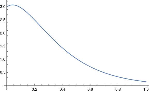
Unlike the case λ > 0, now with λ < 0 the difference between the solutions is bounded. Before the solutions started out close together and eventually diverged. Now the solutions are close together forever.

Here’s a plot of the difference between the two solutions.

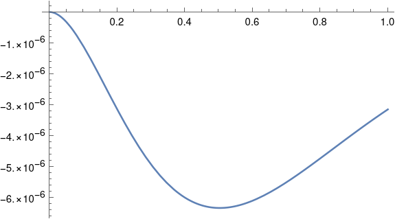
So the maximum separation between the two solutions occurs somewhere around t = 0.5 where the solutions differ in the sixth decimal place.

Conclusion

Whether the characteristic equation has a double root or two close roots makes a significant difference in the written form of the solution to a differential equation. If the roots are positive, the solutions are initially close together then diverge. If the roots are negative, the solutions are always close together.

Difference equations and differential equations

Posted on 12 June 2022 by John

Difference equations are very much analogous to differential equations. Difference equations are more elementary, but differential equations are more familiar.

It seems odd to use a more advanced thing to explain a simpler thing, like saying a quartet is a symphony orchestra with only four instruments. But if for some reason you managed to become familiar with orchestras before learning what a quartet is, this explanation would be helpful.

Differential equations are a standard part of the curriculum for science and engineering students, but difference equations are not. And not without reason: differential equations are a prerequisite for future courses but difference equations are not. But if a curriculum were to include difference equations and differential equations, it might make sense to teach the former first because the topic is more tangible.

To illustrate the similarity between the two topics, this post will solve the difference equation [1]

F_n+2 = F_n+1 + F_n

and the differential equation

y” = y‘ + y

The difference equation defines the Fibonacci numbers, with one set of initial conditions, and the Lucas numbers with different initial conditions. The differential equation is analogous in ways we’ll see below.

Both equations are solved by assuming the form of the solution with a free parameter. Two values of the parameter will be found via a quadratic equation,giving two independent solutions. All solutions are linear combinations of these two solutions.

Difference equation example

The Fibonacci numbers start with F₀ = 0 and F₁ = 1. From there it’s obvious that F₂ = 1, F₃ = 2, and so forth.

The Lucas numbers start with L₀ = 2 and L₁ = 1. From there we see L₂ = 3, L₄ = 4, etc.

Bootstrapping the solution starting from initial conditions is trivial. However, this does not give us a general expression for the solution, and it does not let us explore the solutions of the difference equation for all initial conditions.

So let’s go back and solve the difference equation first, then apply initial conditions, analogous to what one typically does for ordinary differential equations.

Assume solutions have the form F_n = xⁿ for some x to be determined. Then

xⁿ⁺² − xⁿ⁺¹ − xⁿ = 0

for all non-negative n and so

x² − x − 1 = 0

and the two roots are the golden ratio

ϕ = (1 + √5)/2

and its complement

1 − ϕ = (1 − √5)/2.

So the general solution to the recurrence relation

F_n+2 = F_n+1 + F_n

F_n = aϕⁿ + b(1 − ϕ)ⁿ

for constants a and b to be determined by initial conditions. For the Fibonacci numbers, a = 1/√5 and b = −a. For the Lucas numbers, a = b = 1.

Our assumption of the form of the solution is justified because it worked. There can’t be any other solutions of another form because clearly the initial conditions determine the third element of the sequence, and the second and third elements determine the fourth, etc.

Differential equation example

Assume solutions have the form y = exp(kt) for some k to be determined. Sticking this into the differential equation shows

k² exp(kt) − k exp(kt) − exp(kt) = 0

and so

k² − k − 1 = 0.

This is the same equation as above, and so the roots are ϕ and 1 − ϕ. The general solution is

y(t) = a exp(ϕt) + b exp((1−ϕ)t)

where the constants a and b are determined by the initial value of y and y‘.

It’s not as clear in this case that we’ve found all the solutions and that our solution is unique given initial conditions, but it’s true.

[1] Someone might object that this is a recurrence relation and not a difference equation: each term is defined in terms of its predecessors, but not in terms of function differences. But you could rewrite the equation in terms of differences.

If ΔF_n = F_n – F_n−1 then we can rewrite our equation as Δ² F – 3ΔF + F = 0.

Oscillations in RLC circuits

Posted on 2 April 2022 by John

Electrical and mechanical oscillations satisfy analogous equations. This is the basis of using the word “analog” in electronics. You could study a mechanical system by building an analogous circuit and measuring that circuit in a lab.

Mass, dashpot, spring

Years ago I wrote a series of four posts about mechanical vibrations:

Everything in these posts maps over to electrical vibrations with a change of notation.

That series looked at the differential equation

$m u'' + \gamma u' + k u = F \cos\omega t$

where m is mass, γ is damping from a dashpot, and k is the stiffness of a spring.

Inductor, resistor, capacitor

Now we replace our mass, dashpot, and spring with an inductor, resistor, and capacitor.

Imagine a circuit with an L henry inductor, and R ohm resistor, and a C farad capacitor in series. Let Q(t) be the charge in coulombs over time and let E(t) be an applied voltage, i.e. an AC power source.

Charge formulation

One can use Kirchhoff’s law to derive

Here we have the correspondences

$\begin{align*} u &\leftrightarrow Q \\ m &\leftrightarrow L \\ \gamma &\leftrightarrow R \\ k &\leftrightarrow 1/C \end{align*}$

So charge is analogous to position, inductance is analogous to mass, resistance is analogous to damping, and capacitance is analogous to the reciprocal of stiffness.

The reciprocal of capacitance is called elastance, so we can say elastance is proportional to stiffness.

Current formulation

It’s more common to see the differential equation above written in terms of current I.

$I = \frac{dQ}{dt}$

If we take the derivative of both sides of

we get

$LI'' + RI' + \frac{1}{C} I = E'$

Natural frequency

With mechanical vibrations, as shown here, the natural frequency is

$\omega_0 = \sqrt{\frac{k}{m}}$

and with electrical oscillations this becomes

$\omega_0 = \frac{1}{\sqrt{LC}}$

Steady state

When a mechanical or electrical system is driven by sinusoidal forcing function, the system eventually settles down to a solution that is proportional to a phase shift of the driving function.

To be more explicit, the solution to the differential equation

$m u'' + \gamma u' + k u = F \cos\omega t$

has a transient component that decays exponentially and a steady state component proportional to cos(ωt-φ). The same is true of the equation

$LI'' + RI' + \frac{1}{C} I = E'$

The proportionality constant is conventionally denoted 1/Δ and so the steady state solution is

$\frac{F}{\Delta} \cos(\omega t - \phi)$

for the mechanical case and

$\frac{T}{\Delta} \cos(\omega t - \phi)$

for the electrical case.

The constant Δ satisfies

$\Delta^2 = m^2(\omega_0^2 -\omega^2)^2 + \gamma^2 \omega^2$

for the mechanical system and

$\Delta^2 = L^2(\omega_0^2 -\omega^2)^2 + R^2 \omega^2$

for the electrical system.

When the damping force γ or the resistance R is small, then the maximum amplitude occurs when the driving frequency ω is near the natural frequency ω₀.

More on damped, driven oscillations here.

Lyapunov exponents

Posted on 8 February 2022 by John

Chaotic systems are unpredictable. Or rather chaotic systems are not deterministically predictable in the long run.

You can make predictions if you weaken one of these requirements. You can make deterministic predictions in the short run, or statistical predictions in the long run.

Lyapunov exponents are a way to measure how quickly the short run turns into the long run. There is a rigorous definition of a Lyapunov exponent, but I often hear the term used metaphorically. If something is said to have a large Lyapunov exponent, it quickly becomes unpredictable. (Unpredictable as far as deterministic prediction.)

In a chaotic system, the uncertainty around the future state of the system grows exponentially. If you start with a small sphere of initial conditions at time t = 0, a sphere of diameter ε, that sphere becomes an ellipsoid over time. The logarithm of the ratio of the maximum ellipsoid diameter to the diameter of the initial sphere is the Lyapunov exponent λ. (Technically you have to average this log ratio over all possible starting points.)

With a Lyapunov exponent λ the uncertainty in your solution is bounded by ε exp(λt).

You can predict the future state of a chaotic system if one of ε, λ, or t is small enough. The larger λ is, the smaller t must be, and vice versa. So in this sense the Lyapunov exponent tells you how far out you can make predictions; eventually your error bars are so wide as to be worthless.

A Lyapunov exponent isn’t something you can easily calculate exactly except for toy problems, but it is something you can easily estimate empirically. Pick a cloud of initial conditions and see what happens to that cloud over time.

Differential equations

Eliminating terms from higher-order differential equations

Elliptic coordinates and Laplace’s equation

Separation of variables

Confocal elliptic coordinates

Related

Trading generalized derivatives for classical ones

Related posts

A more direct approach to series solutions

Related links

Operator calculus

Abandon hope of originality

The role of rigor

Operator calculus

Is this worth it?

Related posts

Which one is subharmonic?

Related posts

Double roots and ODEs

Double roots

Close roots

Example with λ > 0

Example with λ < 0

Conclusion

More differential equation posts

Difference equations and differential equations

Difference equation example

Differential equation example

Related posts

Oscillations in RLC circuits

Mass, dashpot, spring

Inductor, resistor, capacitor

Charge formulation

Current formulation

Natural frequency

Steady state

Lyapunov exponents

Related posts