A closer look at zero spacing

A few days ago I wrote about Kneser’s theorem. This theorem tells whether the differential equation

u ″(x) + h(x) u(x) = 0

will oscillate indefinitely, i.e. whether it will have an infinite number of zeros.

Today’s post will look at another theorem that gives more specific information about the spacing of the zeros.

Kneser’s theorem said that the growth rate of h determines the oscillatory behavior of the solution u. Specifically, if h grows faster than ¼x−2 then oscillations will continue, but otherwise they will eventually stop.

Zero spacing

A special case of a theorem given in [1] says that an upper bound on h gives a lower bound on zero spacing, and a lower bound on h gives an upper bound on zero spacing.

Specifically, if h is bound above by M, then the spacing between zeros is no more than π/√M. And if h is bound below by M′, then the spacing between zeros is no less than π/√M′.

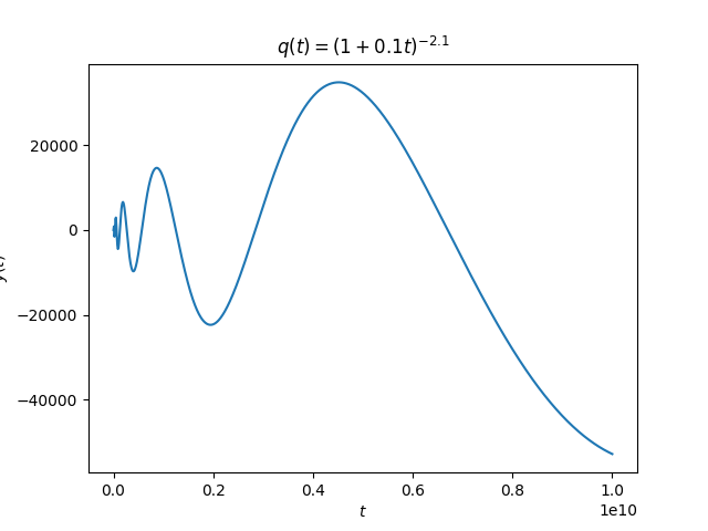
Let’s look back a plot from the post on Kneser’s theorem:

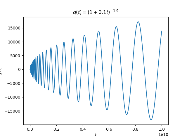
The spacing between the oscillations appears to be increasing linearly. We could have predicted that from the theorem in this post. The coefficient of the linear term is roughly on the order of 1/x² and so the spacing between the zeros is going to be on the order of x.

Specifically, in the earlier post we looked at

h(x) = (1 + x/10)p

where p was 1.9 and 2.1, two exponents chosen to be close to either side of the boundary in Kneser’s theorem. That post used q and t rather than h and x, but I changed notation here to match [1].

Suppose we’ve just seen a zero at x*. Then from that point on h is bounded above by h(x*) and so the distance to the next zero is bounded below by π/√h(x*). That tells you where to start looking for the next zero.

Our function h is bounded below only by 0, and so we can’t apply the theorem above globally. But we could look some finite distance ahead, and thus get a positive lower bound, and that would lead to an upper bound on the location of the next zero. So we could use theory to find an interval to search for our next zero.

More general theorem

The form of the theorem I quoted from [1] was a simplification. The full theorem considers the differential equation

u ″(x) + g(xu′(x) +  h(x) u(x) = 0

The more general theorem looks at upper and lower bounds on

h(x) − ½ g′(x) − ¼ g(x)².

but in our case g = 0 and so the hypotheses reduced to bounds on just h.

Example

Exercise 3 from [1] says to look at the zeros of solution to

u ″(x) + ½x²  u ′ + (10 + 2x) u(x) = 0.

Here we have

h(x) − ½ g ′(x) − ¼ g(x)² = 10 + 2xx − 1  = 9 + x

and so the lower bound of 9 tells us zeros are spaced at most π/3 apart.

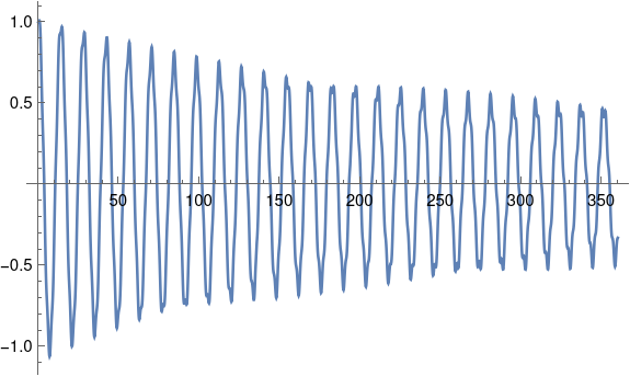
Let’s look at a plot of the solution using Mathematica.

    s = NDSolve[{u''[x] + 0.5 x^2 u'[x] + (10 + 2 x) u[x] == 0, 
                 u[0] == 1, u'[0] == 1 }, u, {x, 0, 5}]
    Plot[Evaluate[u[x] /. s], {x, 0, 5}]

This produces the following.

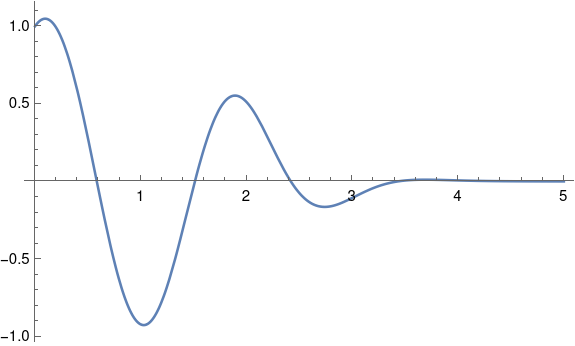
There are clearly zeros between 0 and 1, between 1 and 2, and between 2 and 3. It’s hard to see whether there are any more. Let’s see exactly where the roots are that we’re sure of.

    FindRoot[u[x] /. s, {x, 0, 1}]
    {x -> 0.584153}

    FindRoot[u[x] /. s, {x, 1, 2}]
    {x -> 1.51114}

    FindRoot[u[x] /. s, {x, 2, 3}]
    {x -> 2.41892}

The distance between the first two zeros is 0.926983 and the distance between the second and third zeros is 0.90778. This is consistent with our theorem because π/3 > 1 and the spacing between our zeros is less than 1.

Are there more zeros we can’t see in the plot above? When I asked Mathematica to evaluate

    FindRoot[u[x] /. s, {x, 2, 4}]

it failed with several warning messages. But we know from our theorem that if there is another zero, it has to be less than a distance of π/3 from the last one we found. We can use this information to narrow down where we want Mathematica look.

    FindRoot[u[x] /. s, {x, 2.41892, 2.41892 + Pi/3}]

Now Mathematica says there is indeed another solution.

    {x -> 3.42523}

Is there yet another solution? If so, it can’t be more than a distance π/3 from the one we just found.

    FindRoot[u[x] /. s, {x, 3.42523, 3.42523 + Pi/3}]

This returns 3.42523 again, so Mathematica didn’t find another zero. Assuming Mathematica is correct, this means there cannot be any more zeros.

On the interval [0, 5] the quantity in the theorem is bound above by 14, so an additional zero would need to be at least π/√14 away from the latest one. So if there’s another zero, it’s in the interval [4.26486, 4.47243]. If we ask Mathematica to find a zero in that interval, it fails with warning messages. We can plot the solution over that interval and see that it’s never zero.

[1] Protter and Weinberger. Maximum Principles in Differential Equations. Springer-Verlag. 1984. Page 46.

Slowing oscillations

Consider the second order linear differential equation

y''(t) + ky(t) = 0
You could think of y as giving the height of a mass attached to a spring at time t where k is the stiffness of the spring. The solutions are sines and cosines with frequency √k. Think about how the solution depends on the spring constant k. If k is decreases, corresponding to softening the spring, the frequency of the solutions is decreases, and the period between oscillations increases.

Now suppose we replace the constant k with a decreasing positive function q(t). It seems that by controlling the decay rate of q we could control the oscillations of our system. For q decaying slowly but not too slowly, the solutions would continue to oscillate, crossing back and forth across the zero position, but with increasing time between crossings.

Below some critical rate of decay, the solutions may stop crossing the x axis at all. It seems plausible that if q decreases quickly enough, the period could decrease along with it at just the right rate so that the next oscillation never fully arrives.

Adolf Kneser (1862–1930) proved that the intuition described above is indeed correct. He proved that if

\limsup _{t \to \infty} t^2 q(t) < \frac{1}{4}

the solutions to

y'' + q(t)y = 0

will eventually stop oscillating, but if

\liminf _{t \to \infty} t^2 q(t) > \frac{1}{4}

they will oscillate forever.

Example

We’ll set for initial conditions y(0) = 1 and y ‘(0) = 0.

Let q(t) = (1 + 0.1 t)−1.9.  This choice of q decays slower than 0.25 t−2 and so our solutions should oscillate indefinitely. And that appears to be the case:

The period between zero crossings is increasing, but according to Kneser’s theorem the crossings will never stop.

Next we redo our calculation with q(t) = (1 + 0.1 t)−2.1. Now we’re on the other side of Kneser’s theorem and so we expect oscillations to eventually stop.

There are a lot more zero crossings than are evident in the plot; they just can’t be seen because the horizontal scale is so large.

According to Kneser’s theorem there is a last time the solution crosses zero, and I believe it occurs around 2×1026.

More differential equation posts

Hypergeometric equation

I’ve asserted numerous times here that hypergeometric functions come up very often in applied math, but I haven’t said why. This post will give one reason why.

One way to classify functions is in terms of the differential equations they satisfy. Elementary functions satisfy simple differential equations. For example, the exponential function satisfies

y′ = y

and sine and cosine satisfy

y″ + y = 0.

Second order linear differential equations are common and important because Newton’s are second order linear differential equations. For the rest of the post, differential equations will be assumed to be second order and linear, with coefficients that are analytic except possibly at isolated singularities.

ODEs can be classified in terms of the singularities of their coefficients. The equations above have no singularities and so their solutions are some of the most fundamental equations.

If an ODE has two or fewer regular singular points [1], it can be solved in terms of elementary functions. The next step in complexity is to consider differential equations whose coefficients have three regular singular points. Here’s the kicker:

Every ODE with three regular singular points can be transformed into the hypergeometric ODE.

So one way to think of the hypergeometric differential equation is that it is the standard ODE with three regular singular points. These singularities are at 0, 1, and ∞. If a differential equation has singularities elsewhere, a change of variables can move the singularities to these locations.

The hypergeometric differential equation is

x(x − 1) y″ + (c − (a + b + 1)x) y′ + ab y = 0.

The hypergeometric function F(a, b; c; x) satisfies this equation, and if c is not an integer, then a second independent solution to the equation is

x1−c F(1 + ac, 1 + bc; 2 − c; x).

To learn more about the topic of this post, see Second Order Differential Equations: Special Functions and Their Classification by Gerhard Kristensson.

Related posts

[1] This includes singular points at infinity. A differential equation is said to have a singularity at infinity if under the change of variables t = 1/x the equation in u has a singularity at 0. For example, Airy’s equation

y″ + x y = 0

has no singularities in the finite complex plane, and it has no solution in terms of elementary functions. This does not contradict the statement above because the equation has a singularity at infinity.

Quadruple factorials and Legendre functions

Last week I claimed that double, triple, and quadruple factorials came up in applications. The previous post showed how triple factorials come up in solutions to Airy’s equation. This post will show how quadruple factorials come up in solutions to Legendre’s equation.

Legendre’s differential equation is

(1 - x^2) y^{\prime\prime} -2x y^\prime + \nu(\nu+1)y = 0

The Legendre functions Pν and Qν are independent solutions to the equation for given values of ν.

When ν is of the form n + ½ for an integer n, the values of Pν and Qν at 0 involve quadruple factorials and also Gauss’s constant.

For example, if ν = 1/2, 5/2, 9/2, …, then Pν(0) is given by

(-1)^{(2\nu - 1)/4} \frac{\sqrt{2}(2\nu - 2)!!!!}{(2\nu)!!!!\pi g}

Source:  An Atlas of Functions

Triple factorials and Airy functions

Last week I wrote in a post on multifactorials in which I said that

Double factorials come up fairly often, and sometimes triple, quadruple, or higher multifactorials do too.

This post gives a couple examples of triple factorials in practice.

One example I wrote about last week. Triple factorial comes up when evaluating the gamma function at an integer plus 1/3. As shown here,

\Gamma\left(n + \frac{1}{3}\right) = \frac{(3n-2)!!!}{3^n} \Gamma\left(\frac{1}{3}\right)

Another example involves solutions to Airy’s differential equation

y'' - xy = 0

One pair of independent solutions consists of the Airy functions Ai(x) and Bi(x). Another pair consists of the functions

\begin{align*} f(x) &= 1 + \frac{1}{3!}x^3 + \frac{1\cdot 4}{6!}x^6 + \frac{1\cdot 4 \cdot 7}{9!}x^9 + \cdots \\ g(x) &= x + \frac{2}{4!}x^4 + \frac{2\cdot 5}{7!}x^7 + \frac{2\cdot 5 \cdot 8}{10!}x^{10} + \cdots \end{align*}

given in A&S 10.4.3. Because both pairs of functions solve the same linear ODE, each is a linear combination of the other.

Notice that the numerators are triple factorials, and so the series above can be rewritten as

\begin{align*} f(x) &= \sum_{n=0}^\infty \frac{(3n+1)!!!}{(3n+1)!} x^{3n}\\ g(x) &= \sum_{n=0}^\infty \frac{(3n+2)!!!}{(3n+2)!} x^{3n+1} \end{align*}

The next post gives an example of quadruple factorials in action.

Nonlinear ODEs with stable limit cycles

It’s not obvious when a nonlinear differential equation will have a periodic solution, or asymptotically approach a periodic solution. But there are theorems that give sufficient conditions. This post is about one such theorem.

Consider the equation

x” + f(x) x‘ + g(x) = 0

where f and g are analytic and define F(x) to be the integral of f(t) from 0 to x. The following six hypotheses are sufficient to guarantee that the equation above has a stable limit cycle [1].

  1. g is an odd function,
  2. g is positive for positive x,
  3. f is an even function,
  4. f(o) < 0,
  5. F(x) → ∞ as x → ∞,
  6. F has a unique positive zero.

These hypotheses are satisfied, for example, by Van der Pol’s equation.

Let’s make up coefficient functions f and g that satisfy the conditions above and look for the limit cycle.

We can let g(x) = x³ and f(x) = x² − 1. And here’s what we get:

The graph shows phase portraits for two different initial conditions, given in the legend of the plot. Note that limit cycle appears solid blue because the trajectories of both the dashed line and the dotted line run around the periodic attractor.

Related posts

[1] You can find this theorem in Topics in Ordinary Differential Equations by William Lakin and David Sanchez.

Nonlinear phase portrait

I was reading through Michael Trott’s Mathematica Guidebook for Programming and ran across the following plot.

I find the image aesthetically interesting. I also find it interesting that the image is the phase portrait of a differential equation whose solution doesn’t look that interesting. That is, the plot of (x(t), x ‘(t)) is much more visually interesting than the plot of x(t).

The differential equation whose phase portrait is plotted above is

x''(t) + \frac{1}{20}x'(t)^3 + \frac{1}{5} x(t) = \frac{1}{3}\cos(et)

with initial position 1 and initial velocity 0. It’s a familiar damped, driven harmonic oscillator, except the equation is nonlinear because the derivative term is cubed.

Here’s a plot of the solution as a function of time.

The solution basically looks like the solution of the linear case, except the solutions are more jagged near the local maxima and minima. In fact, the plot looks so jagged that I wondered whether this was an artifact of needing more plotting points. But adding more points didn’t make much difference. Interestingly, although this plot looks jagged, the phase portrait is smooth.

I produced the phase portrait by copying Trott’s code and making a couple small modifications.

    sol = NDSolve[{(*differential equation*)
        x''[t] + 1/20 x'[t]^3 + 1/5 x[t] == 
        1/3 Cos[E t],(*initial conditions*)x[0] == 1, x'[0] == 0}, 
        x, {t, 0, 360}, MaxSteps -> Infinity]

    ParametricPlot[Evaluate[{x[t], x'[t]} /. sol], {t, 0, 360}, 
        Frame -> True, Axes -> False, PlotPoints -> 3600]

Apparently the syntax of NDSolve has changed slightly since Trott’s book was published in 2004. The argument x in the code above was written x[t] in Trott’s original code and this did not work in the current version of Mathematica. I also simplified the call to ParametricPlot slightly, though the original code would work.

Predator-Prey period

The Lotka-Volterra equations are a system of nonlinear differential equations for modeling a predator-prey ecosystem. After a suitable change of units the equations can be written in the form

\begin{align*} \frac{dx}{dt} &= \phantom{-}ax(y-1) \\ \frac{dy}{dt} &= -by(x-1) \end{align}

where ab = 1. Here x(t) is the population of prey at time t and y(t) is the population of predators. For example, maybe x represents rabbits and y represents foxes, or x represents Eloi and y represents Morlocks.

It is well known that the Lotka-Volterra equations have periodic solutions. It is not as well known that you can compute the period of a solution without having to first solve the system of equations.

This post will show how to compute the period of the system. First we’ll find the period by solving the equations for a few different initial conditions, then we’ll show how to directly compute the period from the system parameters.

Phase plot

Here is a plot of (x(t), y(t)) showing that the solutions are periodic.

Predator-prey phase plots for varying initial conditions

And here’s the Python code that made the plot above.

    import matplotlib.pyplot as plt
    import numpy as np
    from scipy.integrate import solve_ivp
    
    # Lotka-Volterra equations
    def lv(t, z, a, b):
        x, y = z
        return [a*x*(y-1), -b*y*(x-1)]
    
    begin, end = 0, 20
    t = np.linspace(begin, end, 300)
    
    styles = ["-", ":", "--"]
    prey_init = [2, 4, 8]
    a = 1.5
    b = 1/a
    
    for style, p0 in zip(styles, prey_init):
        sol = solve_ivp(lv, [begin, end], [p0, 1], t_eval=t, args=(a, b))
        plt.plot(sol.y[0], sol.y[1], style)
    
    plt.xlabel("prey")
    plt.ylabel("preditor")
    plt.legend([f"$p_0$ = {p0}" for p0 in prey_init])    

Note that the derivative of x is zero when y = 1. Since our initial condition sets y(0) = 1, we’re specifying the maximum value of x. (If our initial values of x were less than 1, we’d be specifying the minimum of x.)

Time plot

The components x and y have the same period, and that period depends on a and b, and on the initial conditions. The plot below shows how the period increases with x(0), which as we noted above is the maximum value of x.

Predator-prey solutions over time for varying initial conditions

And here’s the code that made the plot.

    fig, ax = plt.subplots(3, 1)
    for i in range(3):
        sol = solve_ivp(lv, [begin, end], [prey_init[i], 1], t_eval=t, args=(a, b))
        ax[i].plot(t, sol.y[0], "-")
        ax[i].plot(t, sol.y[1], "--")    
        ax[i].set_xlabel("$t$")
        ax[i].set_ylabel("population")
        ax[i].set_title(f"x(0) = {prey_init[i]}")
    plt.tight_layout()

Finding the period

In [1] the author develops a way to compute the period of the system as a function of its parameters without solving the differential equations.

First, calculate an invariant h of the system:

h = b(x - \log(x) - 1) + a(y - \log(y) - 1)

Since this is an invariant we can evaluate it anywhere, so we evaluate it at the initial conditions.

Then the period only depends on a and h. (Recall we said we can scale the equations so that ab = 1, so a and b are not independent parameters.)

If h is not too large, we can compute the approximate period using an asymptotic series.

P(h) = 2\pi\left( 1 + \frac{\sigma}{6} h + \frac{\sigma^2}{144} h^2 + \left(\frac{\sigma}{360} - \frac{139\sigma^3}{38880}\right) h^3 + \cdots \right)

where σ = (a + b)/2 = (a² + 1)/2a.

We use this to find the periods for the example above.

    def find_h(a, x0, y0):
        b = 1/a
        return b*(x0 - np.log(x0) - 1) + a*(y0 - np.log(y0) - 1)

    def P(h, a):
        sigma = 0.5*(a + 1/a)
        s = 1 + sigma*h/6 + sigma**2*h**2/144
        return 2*np.pi*s

    print([P(find_h(1.5, p0, 1), 1.5) for p0 in [2, 4, 8]])

This predicts periods of roughly 6.5, 7.5, and 10.5, which is what we see in the plot above.

When h is larger, the period can be calculated by numerically evaluating an integral given in [1].

Related posts

[1] Jörg Waldvogel. The Period in the Volterra-Lotka Predator-Prey Model. SIAM Journal on Numerical Analysis, Dec., 1983, Vol. 20, No. 6, pp. 1264-1272

Oscillatory differential equations

The solution to a differential equation is called oscillatory if its set of zeros is unbounded. This does not necessarily mean that the solution is periodic, but that it crosses the horizontal axis infinitely often.

Fowler [1] studied the following differential equation demonstrates both oscillatory and nonoscillatory behavior.

x” + tσ |x|γ sgn x = 0

He proved that

  1. If σ + 2 ≥ 0 then all solutions oscillate.
  2. If σ + (γ + 3)/2 < 0 then no solutions oscillate.
  3. If neither (1) nor (2) holds then some solutions oscillate and some do not.

The edge case is σ = -2 and γ = 1. This satisfies condition (1) above. A slight decrease in σ will push the equation into condition (2). And a simultaneous decrease in σ and increase in γ can put it in condition (3).

It turns out that the edge case can be solved in closed form. The equation is linear because γ = 1 and solutions are given by

ct sin(φ + √3 log(t) / 2).

The solutions oscillate because the argument to sine is an unbounded function of t, and so it runs across multiples of π infinitely often. The distance between zero crossings increases exponentially with time because the logarithms of the crossings are evenly spaced.

This post took a different turn after I started writing it. My original intention was to solve the differential equation numerically and say “See: when you change the parameters slightly you get what the theorem says.” But that didn’t work out.

First I tried numerically computing the solution above with σ = −2 and γ = 1, but I didn’t see oscillations. I tried making σ a little larger, but still didn’t see oscillations. When I increased σ more I could see the oscillations.

I was able to go back and see the oscillations with σ = −2 and γ = 1 by tweaking the parameters in my ODE solver. It’s best practice to tweak your parameters even if everything looks right, just to make sure your solution is robust to algorithm changes. Maybe I would have done that, but since I already knew the analytic solution, I knew to tweak the parameters until I saw the right behavior.

Without some theory as a guide, it would be difficult to determine from numerical solutions alone whether a solution oscillates. If you see oscillations, then they’re probably real (unless your numerical method is unstable), but if you don’t see oscillations, how do you know you won’t see them if you look further out? How much further out should you look? In a practical application, the context of your problem will tell you how far out to look.

My intention was to recommend the equation above as an illustration for an introductory DE class because it demonstrates the important fact that small changes to an equation can qualitatively change the behavior of the solutions. This is especially true for nonlinear DEs, which the above equation is when γ ≠ 1. It could still be used for that purpose, but it would make a better demonstration than homework exercise. The instructor could tune the DE solver to make sure the solutions are qualitatively correct.

I recommend the equation as an illustration, but for a course covering numerical solutions to DEs. It illustrates a different point than I first intended, namely the potentially finicky behavior of software for solving differential equations.

There are a couple morals to this story. One is that numerical methods have not eliminated the need for theory. The ideal is to combine analytic and numerical methods. Analytic methods point out qualitative behavior that might be hard to discover numerically. And analytic methods are not likely to produce closed-form solutions for nonlinear DEs.

Another moral is that it’s best to twiddle the parameters to your numerical method to make sure the solution doesn’t qualitatively change. If you’ve adequately computed a solution, computing it again with smaller integration steps shouldn’t make much difference. But if you do see a substantial difference, your first solution probably wasn’t as good as you thought.

Related posts

[1] R. H. Fowler. Further studies of Emden’s and similar differential equations. Quarterly Journal of Mathematics. 2 (1931), pp. 259–288.