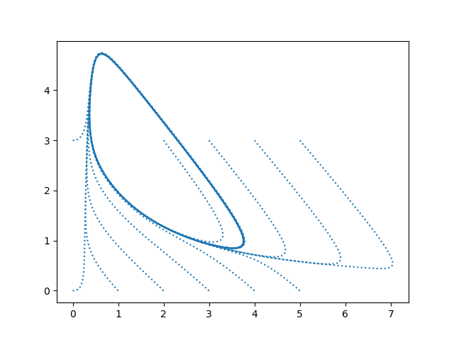
The image below is famous. I’ve seen it many times, but rarely with a detailed explanation. If you’ve ever seen this image but weren’t sure exactly what it means, this post is for you.
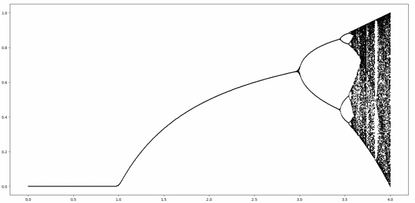
This complex image comes from iterating a simple function
f(x) = r x(1 − x)
known as the logistic map. The iterates of the function can behave differently for different values of the parameter r.
We’ll start by fixing a value of r, with 0 ≤ r < 1. For any starting point 0 ≤ x ≤ 1, f(x) is going to be smaller than x by at least a factor of r, i.e.
0 ≤ f(x) ≤ rx.
Every time we apply f the result decreases by a factor of r.
0 ≤ f( f(x) ) ≤ r²x.
As we do apply f more and more times, the result converges to 0.
For r ≥ 1 it’s not as clear what will happen as we iterate f, so let’s look at a little bit of code to help see what’s going on.
    def f(x, r):
        return r*x*(1-x)

    def iter(x, r, n):
        for _ in range(n):
            x = f(x, r)
        return x
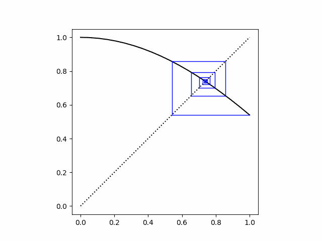
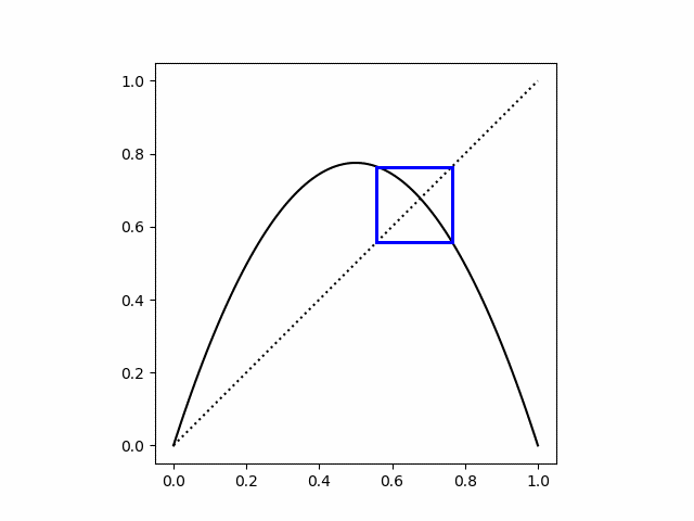
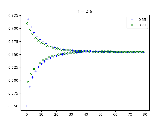
We can see that for 1 ≤ r ≤ 3, and 0 ≤ x ≤ 1, the iterations of f converge to a fixed point, and the value of that fixed point increases with r.
    >>> iter(0.1, 1.1, 100)
    0.09090930810626502

    # more iterations have little effect
    >>> iter(0.1, 1.1, 200)
    0.09090909091486

    # different starting point has little effect
    >>> iter(0.2, 1.1, 200)
    0.0909090909410433

    # increasing r increases the fixed point
    >>> iter(0.2, 1.2, 200)
    0.16666666666666674
Incidentally, for 1 ≤ r ≤ 3, the fixed point equals (r − 1)/r. [1]
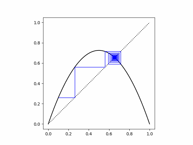
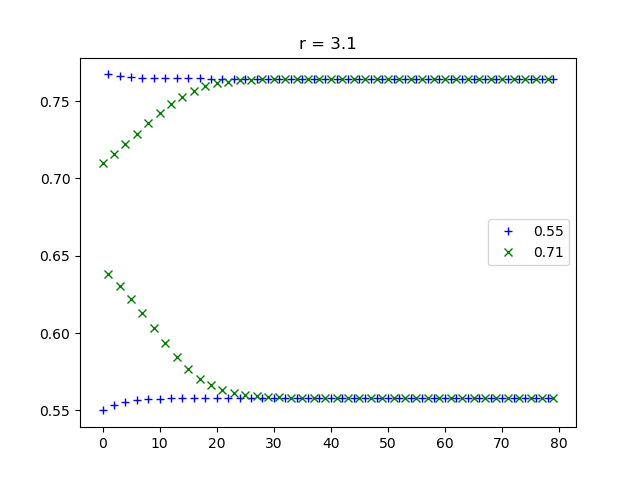
When r is a little bigger than 3, things get more interesting. Instead of a single fixed point, the iterates alternate between a pair of points, an attractor consisting of two points.
    >>> iter(0.2, 3.1, 200)
    0.7645665199585945

    >>> iter(0.2, 3.1, 201)
    0.5580141252026958

    >>> iter(0.2, 3.1, 202)
    0.7645665199585945
How can we write code to detect an attractor? We can look at the set of points when we get, say when we iterate 1000, then 1001, etc. up to 1009 times. If this set has less than 10 elements, the iterates must have returned to one of the values. We’ll round the elements in our set to four digits so we actually get repeated values, not just values that differ by an extremely small amount.
    def attractors(x, r):
        return {round(iter(x, r, n), 4) for n in range(1000,1010)}
This is crude but it’ll do for now. We’ll make it more efficient, and we’ll handle the possibility of more than 10 points in an attractor.
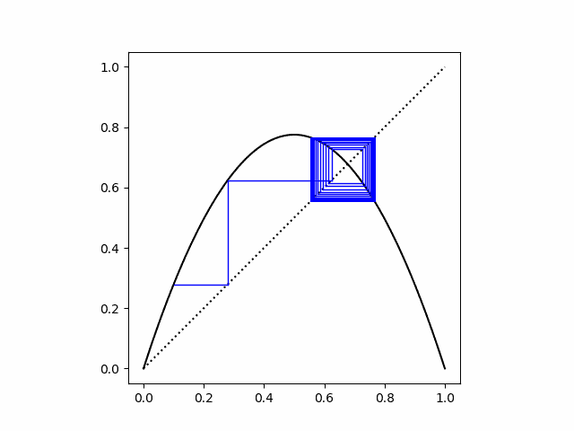
Somewhere around r = 3.5 we get not just two points but four points.
    >>> attractors(0.1, 3.5)
    {0.3828, 0.5009, 0.8269, 0.875}
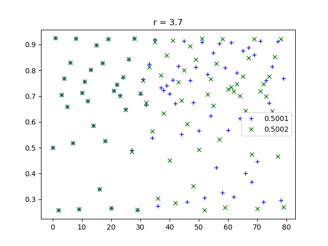
As r gets larger the number of points keeps doubling [2] until chaos sets in.
The function attractors is simple but not very efficient. After doing 1000 iterations, it starts over from scratch to do 1001 iterations etc. And it assumes there are no more than 10 fixed points. The following revision speeds things up significantly.
    def attractors2(x, r):
        x = iter(x, r, 100)
        x0 = round(x, 4)
        ts = {x0}
        for c in range(1000):
            x = f(x, r)
            xr = round(x, 4)
            if xr in ts:
                return ts
            else:
                ts.add(xr)
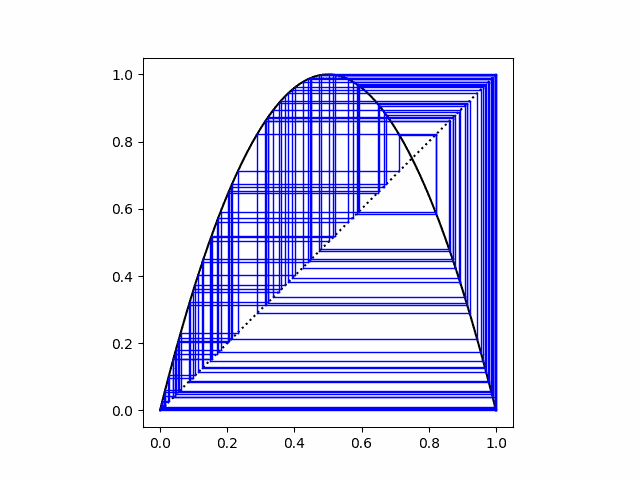
Notice we put a cap of 1000 on the number of points in the attractor for a given r. For some values of r and x, there is no finite set of attracting points.
Finally, here’s the code that produced the image above.
    import numpy as np
    import matplotlib.pyplot as plt
    rs = np.linspace(0, 4, 1000)
    for r in rs:
        ts = attractors2(0.1, r)
        for t in ts:
            plt.plot(r, t, "ko", markersize=1)
    plt.show()
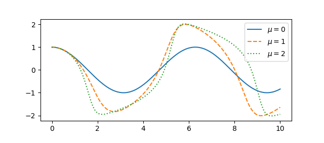
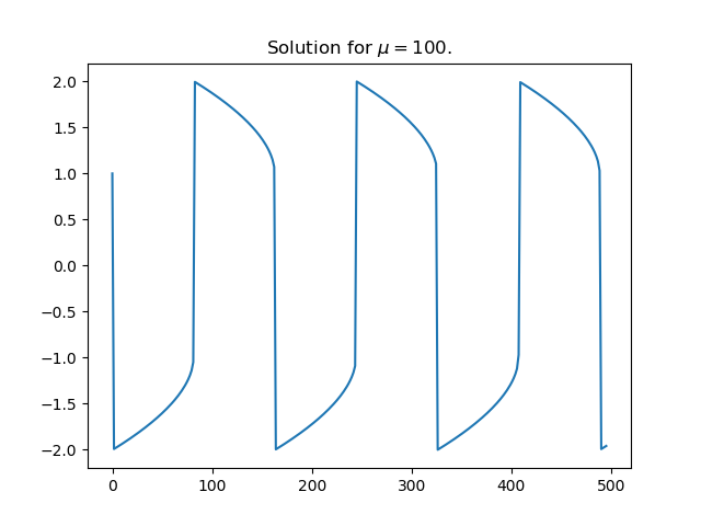
Update: See this post for graphs showing the trajectory of points over time for varying values of r.
More dynamical system posts
[1] Why is this only for 1 ≤ r ≤ 3? Shouldn’t (r − 1)/r be a fixed point for larger r as well? It is, but it’s not a stable fixed point. If x is ever the slightest bit different from (r − 1)/r the iterates will diverge from this point. This post has glossed over some fine points, such as what could happen on a set of measure zero for r > 3.
[2] The spacing between bifurcations decreases roughly geometrically until the system becomes chaotic. The ratio of one spacing to the next reaches a limit known as Feigenbaum’s constant, approximately 4.669. Playing with the code in this post and trying to estimate this constant directly will not get you very far. Feigenbaum’s constant has been computed to many decimal places, but by using indirect methods.