This post will look at two numerical integration methods, the trapezoid rule and Romberg’s algorithm, and memoization. This post is a continuation of ideas from the recent posts on Lobatto integration and memoization.
Although the trapezoid rule is not typically very accurate, it can be in special instances, and Romberg combined it with extrapolation to create a very accurate method.
Trapezoid rule
The trapezoid is the simplest numerical integration method. The only thing that could be simpler is Riemann sums. By replacing rectangles of Riemann sums with trapezoids, you can make the approximation error an order of magnitude smaller.
The trapezoid rule is crude, and hardly recommended for practical use, with two exceptions. It can be remarkably efficient for periodic functions and for analytic functions that decay double exponentially. The trapezoid rule works so well in these cases that it’s common to transform a general function so that it has one of these forms so the trapezoid rule can be applied.
To be clear, the trapezoid rule for a given step size h may not be very accurate. But for periodic and double exponential functions the error decreases exponentially as h decreases.
Here’s an implementation of the trapezoid rule that follows the derivation directly.
    def trapezoid1(f, a, b, n):
        integral = 0
        h = (b-a)/n
        for i in range(n):
            integral += 0.5*h*(f(a + i*h) + f(a + (i+1)*h))
        return integral
This code approximates the integral of f(x) over [a, b] by adding up the areas of n trapezoids. Although we want to keep things simple, a slight change would make this code twice as efficient.
    def trapezoid2(f, a, b, n):
        integral = 0.5*( f(a) + f(b) )
        h = (b-a)/n
        for i in range(1, n):
            integral += f(a + i*h)
        return h*integral
Now we’re not evaluating f twice at every interior point.
Estimating error
Suppose you’ve used the trapezoid rule once, then you decide to use it again with half as large a step size in order to compare the results. If the results are the same within your tolerance, then presumably you have your result. Someone could create a function where this comparison would be misleading, where the two results agree but both are way off. But this is unlikely to happen in practice. As Einstein said, God is subtle but he is not malicious.
If you cut your step size h in half, you double your number of integration points. So if you evaluated your integrand at n points the first time, you’ll evaluate it at 2n points the second time. But half of these points are duplicates. It would be more efficient to save the function evaluations from the first integration and reuse them in the second integration, only evaluating your function at the n new integration points.
It would be most efficient to write your code to directly save previous results, but using memoization would be easier and still more efficient than redundantly evaluating your integrand. We’ll illustrate this with Python code.
Now let’s integrate exp(cos(x)) over [0, π] with 4 and then 8 steps.
    from numpy import exp, cos, pi

    print( trapezoid2(f, 0, pi, 4) )
    print( trapezoid2(f, 0, pi, 8) )
This prints
    3.97746388
    3.97746326
So this suggests we’ve already found our integral to six decimal places. Why so fast? Because we’re integrating a periodic function. If we repeat our experiment with exp(x) we see that we don’t even get one decimal place agreement. The code
    print( trapezoid2(exp, 0, pi, 4 ) )
    print( trapezoid2(exp, 0, pi, 8 ) )
prints
    23.26
    22.42
Eliminating redundancy
The function trapezoid2 eliminated some redundancy, but we still have redundant function evaluations when we call this function twice as we do above. When we call trapezoid2 with n = 4, we do 5 function evaluations. When we call it again with n = 8 we do 9 function evaluations, 4 of which we’ve done before.
As we did in the Lobatto quadrature example, we will have our integrand function sleep for 10 seconds to make the function calls obvious, and we will add memoization to have Python to cache function evaluations for us.
    from time import sleep, time
    from functools import lru_cache

    @lru_cache()
    def f(x):
        sleep(10)
        return exp(cos(x))

    t0 = time()
    trapezoid2(f, 0, pi, 4)
    t1 = time()
    print(t1 - t0)
    trapezoid2(f, 0, pi, 8)
    t2 = time()
    print(t2 - t1)
This shows that the first integration takes 50 seconds and the second requires 40 seconds. The first integration requires 5 function evaluations and the second requires 9, but the latter is faster because it only requires 4 new function evaluations.
Romberg integration
In the examples above, we doubled the number of integration intervals and compared results in order to estimate our numerical integration error. A natural next step would be to double the number of intervals again. Maybe by comparing three integrations we can see a pattern and project what the error would be if we did more integrations.
Werner Romberg took this a step further. Rather than doing a few integrations and eye-balling the results, he formalized the inference using Richardson extrapolation to project where the integrations are going. Specifically, his method applies the trapezoid rule at 2m points for increasing values of m. The method stops when either the maximum value of m has been reached or the difference between successive integral estimates is within tolerance. When Romberg’s method is appropriate, it converges very quickly and there is no need for m to be large.
To illustrate Romberg’s method, let’s go back to the example of integrating exp(x) over [0, π]. If we were to use the trapezoid rule repeatedly, we would get these results.
     Steps    Results
         1  37.920111
         2  26.516336
         4  23.267285
         8  22.424495
        16  22.211780
        32  22.158473
This doesn’t look promising. We don’t appear to have even the first decimal correct. But Romberg’s method applies Richardson extrapolation to the data above to produce a very accurate result.
    from scipy.integrate import romberg

    r = romberg(exp, 0, pi, divmax = 5)
    print("exact:   ", exp(pi) - 1)
    print("romberg: ", r)
This produces
    exact:    22.1406926327792
    romberg:  22.1406926327867
showing that although none of the trapezoid rule estimates are good to more than 3 significant figures, the extrapolated estimate is good 12 figures, almost to 13 figures.
If you pass the argument show=True to romberg you can see the inner workings of the integration, including a report that the integrand was evaluated 33 times, i.e. 1 + 2m times when m is given by divmax.
It seems mysterious how Richardson extrapolation could take the integral estimates above, good to three figures, and produce an estimate good to twelve figures. But if we plot the error in each estimate on a log scale it becomes more apparent what’s going on.
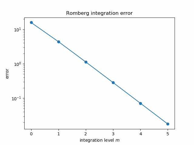
The errors follow nearly a straight line, and so the extrapolated error is “nearly” negative infinity. That is, since the log errors nearly follow a straight line going down, polynomial extrapolation produces a value whose log error is very large and negative.
More on numerical integration