When we say that the planets in our solar system orbit the sun, not the earth, we mean that the motions of the planets is much simpler to describe from the vantage point of the sun. The sun is no more the center of the universe than the earth is. Describing the motion of the planets from the perspective of our planet is not wrong, but it is inconvenient. (For some purposes. It’s quite convenient for others.)
The word planet means “wanderer.” This because the planets appear to wander in the night sky. Unlike stars that appear to orbit the earth in a circle as the earth orbits the sun, planets appear to occasionally reverse course. When planets appear to move backward this is called retrograde motion.
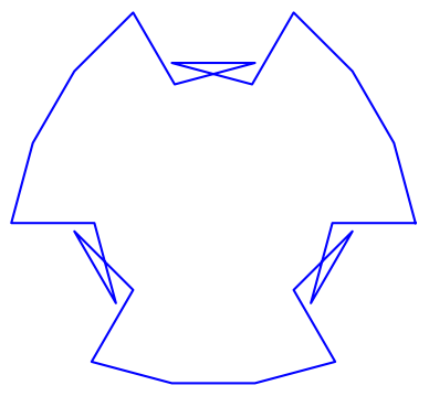
Apparent motion of Venus
Here’s what the motion of Venus would look like over a period of 8 years as explored here.
Venus completes 13 orbits around the sun in the time it takes Earth to complete 8 orbits. The ratio isn’t exactly 13 to 8, but it’s very close. Five times over the course of eight years Venus will appear to reverse course for a few days. How many days? We will get to that shortly.
When we speak of the motion of the planets through the night sky, we’re not talking about their rising and setting each day due to the rotation of the earth on its axis. We’re talking about their motion from night to night. The image above is how an observer far above the Earth and not rotating with the Earth would see the position of Venus over the course of eight years.
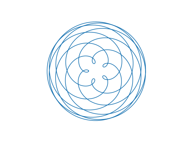
The orbit of Venus as seen from earth is beautiful but complicated. From the Copernican perspective, the orbits of Earth and Venus are simply concentric circles. You may bristle at my saying planets have circular rather than elliptical orbits [1]. The orbits are not exactly circles, but are so close to circular that you cannot see the difference. For the purposes of this post, we’ll assume planets orbit the sun in circles.
Calculating retrograde periods
There is a surprisingly simple equation [2] for finding the points where a planet will appear to change course:

Here r is the radius of Earth’s orbit and R is the radius of the other planet’s orbit [3]. The constant k is the difference in angular velocities of the two planets. You can solve this equation for the times when the apparent motion changes.
Note that the equation is entirely symmetric in r and R. So Venusian observing Earth and an Earthling observing Venus would agree on the times when the apparent motions of the two planets reverse.
Example calculation
Let’s find when Venus enters and leaves retrograde motion. Here are the constants we need.
r = 1       # AU
R = 0.72332 # AU

venus_year = 224.70 # days
earth_year = 365.24 # days
k = 2*pi/venus_year - 2*pi/earth_year

c = sqrt(r*R) / (r + R - sqrt(r*R))
With these constants we can now plot cos(kt) and see when it equals c.
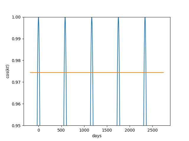
This shows there are five times over the course of eight years when Venus is in apparent retrograde motion.
If we set time t = 0 to be a time when Earth and Venus are aligned, we start in the middle of retrograde period. Venus enters prograde motion 21 days later, and the next retrograde period begins at day 563. So out of every 584 days, Venus spends 42 days in retrograde motion and 542 days in prograde motion.
Related posts
[1] Planets do not exactly orbit in circles. They don’t exactly orbit in ellipses either. Modeling orbits as ellipses is much more accurate than modeling orbits as circles, but not still not perfectly accurate.
[2] 100 Great Problems of Elementary Mathematics: Their History and Solution. By Heinrich Dörrie. Dover, 1965.
[3] There’s nothing unique about observing planets from Earth. Here “Earth” simply means the planet you’re viewing from.