Calculating square roots

Posted on 3 April 2021 by John

Here’s a simple way to estimate the square root of a number x. Take a guess g at the root and compute the average of g and x/g.

If you want to compute square roots mentally or with pencil and paper, how accurate can you get with this method? Could you, for example, get within 1%?

Initial guess

Obviously the answer depends on your guess. One way to form an initial guess is to round x up to the nearest square and take the root of that as your guess. In symbols, we take ⌈√x⌉ as our guess.

For example, if x = 38, you could take 7 as your guess since 49 is the next square after 38. In that case you’d get

(7 + 38/7)/2 = 6.214

The correct value to three places is 6.164, so our error is about 0.8%.

But we could do better. 38 is much closer to 36 than to 49, so we could take 6 as our initial guess. That is, ⌊√38⌋. Then we have

(6 + 38/6) = 6.167

and our relative error is less than 0.04%.

We’ll look at three strategies:

⌊√x⌋
⌈√x⌉
⌊√x⌋ or ⌈√x⌉

In strategy 3, we choose the guess whose square is closer to x.

Initial accuracy

Here’s what we get when we use the method above to estimate the square roots of the numbers from 1 to 100.

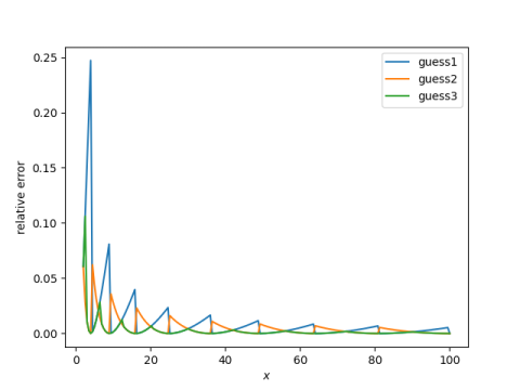
Guess 1 has maximum error 15.5%, where as guess 2 and guess 3 have maximum error 6%.

Guess 2, taking the ceiling, is generally better than guess 1, taking the floor. But guess 3, taking the better of the two, is even better.

More important than which of the three methods used to find the initial guess is being closer to the far end of the range. We could assume x is between 25 and 100 if we first multiply x by a square if necessary to get it into that range. To find the square root of 13, for example, we multiply by 4 and calculate the square root of 13 as half the square root of 52.

If we assume x is between 25 and 100, the maximum errors for the three initial guess methods are 1.4%, 1.3%, and 0.4%.

So to answer our initial question, yes, you can get relative error less than 1%, but you have to do a couple things. You have to multiply by a square to get your number into the range [25, 100] and you have to use the third method of guessing a starting approximation.

Initial and final error

You don’t have to move your number into the range [25, 100] if you put a little more effort into your initial guess. In the example of x = 13 mentioned above, multiplying by 4 before taking the square root is essentially the same as taking 7/2 as your initial guess for √13 instead of using 3 or 4 as an initial guess.

In short, our discussion of the range on x was really a discussion of initial error in disguise. The size of x determines the quality of our initial guesses, but the size of x itself doesn’t matter to the relative error.

Here’s a plot of the final error as a function of the error in the initial guess.

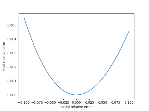
Notice two things. First, the final error is roughly proportional to the square of the error in the initial guess. Second, it’s a little better to guess high than to guess low, which explains why the second method above for guessing starting points is a little better than the first.

Iteration

Another way to get more accuracy is to repeat our process. That is, after we find our estimate, we use it as a new guess and apply our method again. For example, suppose we want to compute the square root of 30. We would find

(5 + 30/5)/2 = 5.5
(5.5 + 30/5.5)/2 = 5.47727

which is correct to four decimal places

We can find square roots to any accuracy we wish by applying this method enough times. In fact, what we’re doing is applying a special case Newton’s root-finding method.

We showed above that the error after each iteration is on the order of the square of the previous error. So roughly speaking, each iteration doubles the number of correct decimal places.

Higher-order roots

See the next post for an analogous method for computing cube roots and nth roots in general.

Computing Fourier series coefficients with the FFT

Posted on 20 March 2021 by John

The Discrete Fourier Transform (DFT) is a mathematical function, and the Fast Fourier Transform (FFT) is an algorithm for computing that function. Since the DFT is almost always computed via the FFT, the distinction between the two is sometimes lost.

It is often not necessary to distinguish between the two. In my previous post, I used the two terms interchangeably because the distinction didn’t matter in that context.

Here I will make a distinction between the DFT and the FFT; I’ll use DFT to refer to the DFT as it is defined in [1], and FFT for the DFT as computed in NumPy‘s FFT routine. The differences are due to varying conventions; this is often an issue.

Suppose we have a function f on an interval [−A/2, A/2] and we sample f at N points where N is an even integer.

Define

$\begin{align*} \Delta x &= A/N \\ x_n &= n \Delta x \\ f_n &= f(x_n) \end{align*}$

for n running from −N/2 + 1 to N/2.

DFT of the sequence {f_n} is defined in [1] as the sequence {F_k} where

$F_k = \frac{1}{N}\sum_{n = -N/2 + 1}^{N/2} f_n \exp(-2 \pi i n k/N)$

Now suppose the function f that we sampled has a Fourier series

$f(x) = \sum_{k = -\infty}^\infty c_k \exp(2 \pi i k x/A)$

The Fourier coefficients c_k relate to the DFT output F_k according to the Discrete Poisson Summation Formula [1]:

$F_k = c_k + \sum_{j=-\infty}^\infty \left(c_{k+jN} - c_{k-jN}\right)$

This means that the c_k simply equal the F_k if f has no frequency components higher than N/2 Hz because all the terms in the infinite sum above are zero. That is, if f is band-limited and we have sampled at a frequency higher than the Nyquist frequency, then we can simply read the Fourier coefficients off the DFT.

However, when f is not band-limited, or when it is band-limited but we have not sampled it finely enough, we will have aliasing. Our Fourier coefficients will differ from our DFT output by an error term involving high-frequency Fourier series coefficients.

In application it’s usually too much to hope that your function is exactly band-limited, but it may be approximately band-limited. The Fourier coefficients of smooth functions eventually decay rapidly (see details here) and so the error in approximating Fourier series coefficients by DFT terms is small.

Computing a DFT with the FFT

We defined the DFT of the sequence {f_n} above to be the sequence {F_k} where

$F_k = \frac{1}{N}\sum_{n = -N/2 + 1}^{N/2} f_n \exp(-2 \pi i n k/N)$

and k runs from −N/2 + 1 to N/2.

NumPy, on the other hand, defines the DFT of the sequence {a_n} to be the sequence {A_k} where

$A_k = \sum_{n = 0}^{N-1} a_n \exp(-2 \pi i n k/N)$

and k runs from 0 to N − 1.

Relative to the definition in the previous post, the NumPy definition difference in three ways:

The normalization factor 1/N is missing.
The input indices are numbered differently.
The output is arranged differently.

The first difference is trivial to overcome: simply divide the FFT output by N.

The second difference is easy to deal with if we think of the inputs to the FFT being samples from a periodic function, which they usually are. The f_k come from sampling a periodic function f over an interval [−A/2, A/2]. If we sample the same function over [0, A] we get the a_n. We have

$\begin{align*} f(0) &= f_0 = a_0 \\ f(A/N) &= f_1 = a_1 \\ f(2A/N) &= f_2 = a_2 \\ \cdots \\ f(A) &= f_{N/2} = a_{N/2} \end{align*}$

If we extend the fs and the as periodically past their original ranges of definition, then they all agree. But since we start our sampling in difference places, our samples would be listed in different orders if we stored them by increasing index.

Something similar occurs with the output.

For 0 ≤ k ≤ N/2,

F_k = A_k.

But for N < k < N,

F_k = A_N−k.

Example

We’ll use a band-limited function in our example so that we find the Fourier coefficients exactly.

f(x) = 7 cos(6πx) − 5 sin(4πx)

We compute the FFT as follows.

    import numpy as np

    def f(x):
        return 7*np.sin(3*2*np.pi*x) - 5*np.cos(2*2*np.pi*x)

    N = 8
    delta = 1/N
    x = [f(n*delta) for n in range(N)]
    print( np.fft.fft(x)/N )

The output is

[0, 0, −2.5, −3.5i, 0, 3.5i, −2.5, 0]

This says F₂ and F₋₂ = −5/2, and so the coefficient of cos(2·2πx) is −5.

Also F₃ = −7/2 and F₋₃ = 7/2, so the coefficient of cos(3·2πx) is 7. These results follow from Euler’s equation

exp(iθ) = cos(θ) + i sin(θ)

[1] William L. Briggs and Van Emden Henson. The DFT: An Owner’s Manual for the Discrete Fourier Transform. SIAM 1995.

Peaks of Sinc

Posted on 18 January 2021 by John

Yesterday I wrote two posts about finding the peaks of the sinc function. Both focused on numerical methods, the first using a contraction mapping and the second using Newton’s method. This post will focus on the locations of the peaks rather than ways of computing them.

The first post included this discussion of the peak locations.

The peaks of sin(x)/x are approximately at the same positions as sin(x), and so we use (2n + 1/2)π as our initial guess. In fact, all our peaks will be a little to the left of the corresponding peak in the sine function because dividing by x pulls the peak to the left. The larger x is, the less it pulls the root over.

This post will refine the observation above. The paragraph above suggests that for large n, the nth peak is located at approximately (2n + 1/2)π. This is a zeroth order asymptotic approximation. Here we will give a first order asymptotic approximation.

For a fixed positive n, let

θ = (2n + 1/2)π

and let

x = θ + ε

be the location of the nth peak. We will improve or approximation of the location of x by estimating ε.

As described in the first post in this series, setting the derivative of the sinc function to zero says x satisfies

x cos x − sin x = 0.

Therefore

(θ + ε) cos(θ + ε) = sin(θ + ε)

Applying the sum-angle identities for sine and cosine shows

(θ + ε) (cos θ cos ε − sin θ sin ε) = sin θ cos ε + cos θ sin ε

Now sin θ = 1 and cos θ = 0, so

−(θ + ε) sin ε = cos ε.

tan ε = −1/(θ + ε).

So far our calculations are exact. You could, for example, solve the equation above for ε using a numerical method. But now we’re going to make a couple very simple approximations [1]. On the left, we will approximate tan ε with ε. On the right, we will approximate ε with 0. This gives us

ε ≈ −1/θ = −1/(2n + 1/2)π.

This says the nth peak is located at approximately

θ − 1/θ

where θ = (2n + 1/2)π. This refines the earlier statement “our peaks will be a little to the left of the corresponding peak in the sine function.” As n gets larger, the term we subtract off gets smaller. This makes the statement above “The larger x is, the less it pulls the root over” more precise.

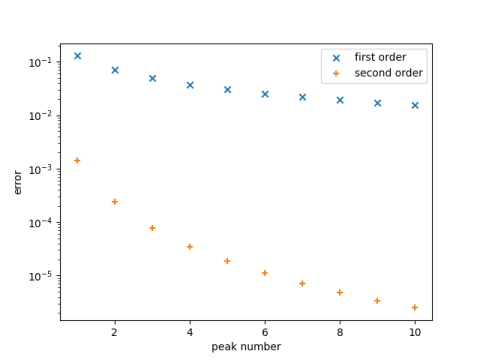
Now let’s see visually how well our approximation works. The graph below plots the error in approximating the nth peak location by θ and by θ – 1/θ.

Note the log scale. The error in approximating the location of the 10th peak by 20.5π is between 0.1 and 0.01, and the error in approximating the location by 20.5π − 1/20.5π is approximately 0.000001.

[1] As pointed out in the comments, you could a slightly better approximation by not being so simple. Instead of approximating 1/(θ + ε) by 1/θ you could use 1/θ − ε/θ² and solve for ε.

Rate of convergence for Newton’s method

Posted on 17 January 2021 by John

In the previous post I looked at the problem of finding the peaks of the sinc function.

In this post we use this problem to illustrate how two formulations of the same problem can behave very differently with Newton’s method.

The previous post mentioned finding the peaks by solving either

x cos x − sin x = 0

or equivalently

tan x − x = 0

It turns out that the former is much better suited to Newton’s method. Newton’s method applied to the first equation will converge quickly without needing to start particularly close to the root. Newton’s method applied to the second equation will fail to converge at all unless the method beings close to the root, and even then the method may not be accurate.

Here’s why. The rate of convergence in solving

f(x) = 0

with Newton’s method is determined by the ratio of the second derivative to the first derivative

| f ‘ ‘ (x) / f ‘ (x) |

near the root.

Think of the second derivative as curvature. Dividing by the first derivative normalizes the scale. So convergence is fast when the curvature relative to the scale is small. Which makes sense intuitively: When a function is fairly straight, Newton’s method zooms down to the root. When a function is more curved, Newton’s method requires more steps.

The following table gives the absolute value of the ratio of the second derivative to the first derivative at the first ten peaks, using both equations. The bound on the error in Newton’s method is proportional to this ratio.

    |------+------------+------------|
    | peak | Equation 1 | Equation 2 |
    |------+------------+------------|
    |    1 |      0.259 |       15.7 |
    |    2 |      0.142 |       28.3 |
    |    3 |      0.098 |       40.8 |
    |    4 |      0.075 |       53.4 |
    |    5 |      0.061 |       66.0 |
    |    6 |      0.051 |       78.5 |
    |    7 |      0.044 |       91.1 |
    |    8 |      0.039 |      103.7 |
    |    9 |      0.034 |      116.2 |
    |   10 |      0.031 |      128.8 |
    |------+------------+------------|

The error terms are all small for the first equation, and they get smaller as we look at peaks further from the origin. The error terms for the second equation are all large, and get larger as we look at peaks further out.

For the third and final post in this series, see Peaks of Sinc.

Reverse iteration root-finding

Posted on 17 January 2021 by John

The sinc function is defined by

sinc(x) = sin(x)/x.

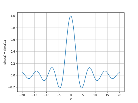
This function comes up constantly in signal processing. Here’s a plot.

We would like to find the location of the function’s peaks. Let’s focus first on the first positive peak, the one that’s somewhere between 5 and 10. Once we can find that one, the rest will be easy.

If you take the derivative of sinc and set it to zero, you find that the peaks must satisfy

x cos x – sin x = 0

which means that

tan x = x.

So our task reduces to finding the fixed points of the tangent function. One way to find fixed points is simply to iterate the function. We pick a starting point near the peak we’re after, then take its tangent, then take the tangent of that, etc.

The peak appears to be located around 7.5, so we’ll use that as a starting point. Then iterates of tangent give

     2.7060138667726910
    -0.4653906051625444
    -0.5021806478408769
    -0.5491373258198057
    -0.6119188887713993
    -0.7017789436750164
    -0.8453339618848119
    -1.1276769374114777
    -2.1070512803092996
     1.6825094538261074

That didn’t work at all. That’s because tangent has derivative larger than 1, so it’s not a contraction mapping.

The iterates took us away from the root we were after. This brings up an idea: is there some way to iterate a negative number of times? Well, sorta. We can run our iteration backward.

Instead of solving

tan x = x

we could equivalently solve

arctan x = x.

Since iterating tangent pushes points away, iterating arctan should bring them closer. In fact, the derivative of arctan is less than 1, so it is a contraction mapping, and we will get a fixed point.

Let’s start again with 7.5 and iterate arctan. This quickly converges to the peak we’re after.

    7.721430101677809
    7.725188823982156
    7.725250798474231
    7.725251819823800
    7.725251836655669
    7.725251836933059
    7.725251836937630
    7.725251836937706
    7.725251836937707
    7.725251836937707

There is a little complication: we have to iterate the right inverse tangent function. Since tangent is periodic, there are infinitely many values of x that have a particular tangent value. The arctan function in NumPy returns a value between -π/2 and π/2. So if we add 2π to this value, we get values in an interval including the peak we’re after.

Here’s how we can find all the peaks. The peak at 0 is obvious, and by symmetry we only need to find the positive peaks; the nth negative peak is just the negative of the nth positive peak.

The peaks of sin(x)/x are approximately at the same positions as sin(x), and so we use (2n + 1/2)π as our initial guess. In fact, all our peaks will be a little to the left of the corresponding peak in the sine function because dividing by x pulls the peak to the left. The larger x is, the less it pulls the root over.

The following Python code will find the nth positive peak of the sinc function.

    def iterate(n, num_iterates = 6):
        x = (2*n + 0.5)*np.pi
        for _ in range(num_iterates):
            x = np.arctan(x) + 2*n*np.pi
    return x

My next post will revisit the problem in this post using Newton’s method.

Symplectic Euler

Posted on 12 September 2020 by John

This post will look at simple numerical approaches to solving the predator-prey (Lotka-Volterra) equations. It turns out that the simplest approach does poorly, but a slight variation does much better.

Following [1] we will use the equations

u‘ = u (v − 2)
v‘ = v (1 − u)

Here u represents the predator population over time and v represents the prey population. When the prey v increase, the predators u increase, leading to a decrease in prey, which leads to a decrease in predators, etc. The exact solutions are periodic.

Euler’s method replaces the derivatives with finite difference approximations to compute the solution in increments of time of size h. The explicit Euler method applied to our example gives

u(t + h) = u(t) + h u(t) (v(t) − 2)
v(t + h) = v(t) + h v(t) (1 − u(t)).

The implicit Euler method gives

u(t + h) = u(t) + h u(t + h) (v(t + h) − 2)
v(t + h) = v(t) + h v(t + h) (1 − u(t + h)).

This method is implicit because the unknowns, the value of the solution at the next time step, appear on both sides of the equation. This means we’d either need to do some hand calculations first, if possible, to solve for the solutions at time t + h, or use a root-finding method at each time step to solve for the solutions.

Implicit methods are more difficult to implement, but they can have better numerical properties. See this post on stiff equations for an example where implicit Euler is much more stable than explicit Euler. I won’t plot the implicit Euler solutions here, but the implicit Euler method doesn’t do much better than the explicit Euler method in this example.

It turns out that a better approach than either explicit Euler or implicit Euler in our example is a compromise between the two: use explicit Euler to advance one component and use implicit Euler on the other. This is known as symplectic Euler for reasons I won’t get into here but would like to discuss in a future post.

If we use explicit Euler on the predator equation but implicit Euler on the prey equation we have

u(t + h) = u(t) + h u(t) (v(t + h) − 2)
v(t + h) = v(t) + h v(t + h) (1 − u(t)).

Conversely, if we use implicit Euler on the predator equation but explicit Euler on the prey equation we have

u(t + h) = u(t) + h u(t + h) (v(t) − 2)
v(t + h) = v(t) + h v(t) (1 − u(t + h)).

Let’s see how explicit Euler compares to either of the symplectic Euler methods.

First some initial setup.

    import numpy as np

    h  = 0.08  # Step size
    u0 = 6     # Initial condition
    v0 = 2     # Initial condition
    N  = 100   # Numer of time steps

    u = np.empty(N)
    v = np.empty(N)
    u[0] = u0
    v[0] = v0

Now the explicit Euler solution can be computed as follows.

    for n in range(N-1):
        u[n+1] = u[n] + h*u[n]*(v[n] - 2)
        v[n+1] = v[n] + h*v[n]*(1 - u[n])

The two symplectic Euler solutions are

    
    for n in range(N-1):
        v[n+1] = v[n]/(1 + h*(u[n] - 1))
        u[n+1] = u[n] + h*u[n]*(v[n+1] - 2)

and

    for n in range(N-1):
        u[n+1] = u[n] / (1 - h*(v[n] - 2))
        v[n+1] = v[n] + h*v[n]*(1 - u[n+1])

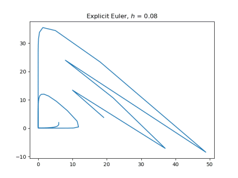
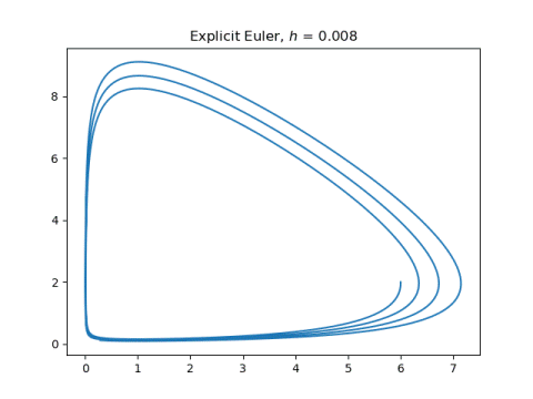
Now let’s see what our solutions look like, plotting (u(t), v(t)). First explicit Euler applied to both components:

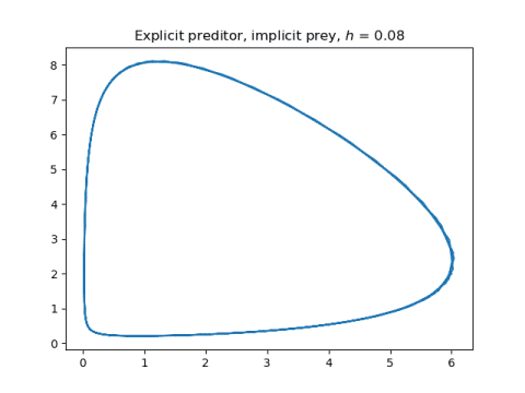
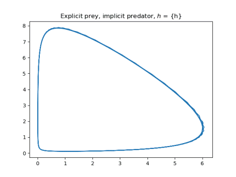
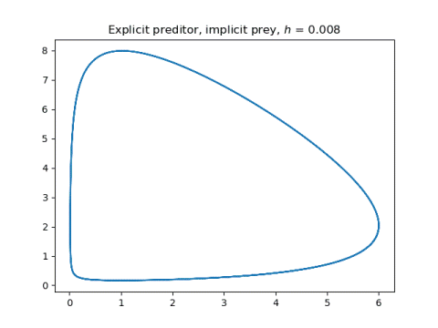
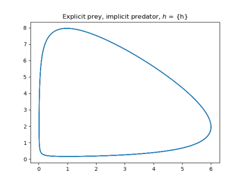
And now the two symplectic methods, applying explicit Euler to one component and implicit Euler to the other.

Next, let’s make the step size 10x smaller and the number of steps 10x larger.

Now the explicit Euler method does much better, though the solutions are still not quite periodic.

The symplectic method solutions hardly change. They just become a little smoother.

Conceptual vs Numerical

Posted on 3 August 2020 by John

One of the things that makes numerical computation interesting is that it often reverses the usual conceptual order of things, using advanced math to compute things that are introduced earlier.

Here’s an example I recently ran across [1]. The hyperbolic functions are defined in terms of the exponential function:

$\begin{align*} \sinh(x) &= \frac{\exp(x) - \exp(-x)}{2} \\ \cosh(x) &= \frac{\exp(x) + \exp(-x)}{2} \\ \tanh(x) &= \frac{\exp(x) - \exp(-x)}{\exp(x) + \exp(-x)} \\ \end{align*}$

But it may be more efficient to compute the exponential function in terms of hyperbolic functions. Specifically,

$\exp(x) = \sinh(x) + \sqrt{\sinh(x)^2 + 1}$

Why would you want to compute the simple thing on the left in terms of the more complicated thing on the right? Because hyperbolic sine is an odd function. This means that half its power series coefficients are zero: an odd function only has odd powers in its power series.

Suppose you need to compute the exponential function in an environment where you only have a limited number of registers to store constants. You can get more accuracy out of the same number of registers by using them to store coefficients in the power series for hyperbolic sine than for exp.

If we store n coefficients for sinh, we can include powers of x up to 2n − 1. And since the coefficient of x²ⁿ is zero, the error in our Taylor approximation is O(x²ⁿ⁺¹). See this post for more on this trick.

If we stored n coefficients for exp, we could include powers of x up to n − 1, and our error would be O(xⁿ).

To make things concrete, suppose n = 3 and x = 0.01. The error in the exp function would be on the order of 10⁻⁶, but the error in the sinh function would be on the order of 10⁻¹⁴. That is, we could almost compute exp to single precision and sinh to almost double precision.

(I’m glossing over a detail here. Would you really need to store, for example, the 1 coefficient in front of x in either series? For simplicity in the argument above I’ve implicitly said yes. Whether you’d actually need to store it depends on the details of your implementation.)

The error estimate above uses big-oh arguments. Let’s do an actual calculation to see what we get.

    from math import exp, sinh, sqrt
    
    def exp_taylor(x):
        return 1 + x + 0.5*x**2
    
    def sinh_taylor(x):
        return x + x**3/6 + x**5/120
    
    def exp_via_sinh(x):
        s = sinh_taylor(x)
        return s + sqrt(s*s + 1)
    
    def print_error(approx, exact):
        print(f"Computed: {approx}")
        print(f"Exact:    {exact}")
        print(f"Error:    {approx - exact}")
    
    x = 0.01
    approx1 = exp_taylor(x)
    approx2 = exp_via_sinh(x)
    exact   = exp(x)
    
    print("Computing exp directly:\n")
    print_error(approx1, exact)
    
    print()
    
    print("Computing exp via sinh:\n")
    print_error(approx2, exact)

This produces

    Computing exp directly:

    Computed: 1.0100500000000001
    Exact:    1.010050167084168
    Error:    -1.6708416783473012e-07

    Computing exp via sinh:

    Computed: 1.0100501670841682
    Exact:    1.010050167084168
    Error:    2.220446049250313e-16

Our errors are roughly what we expected from our big-oh arguments.

Leapfrog integrator

Posted on 13 July 2020 by John

The so-called “leapfrog” integrator is a numerical method for solving differential equations of the form

where x is a function of t. Typically x is position and t is time.

This form of equation is common for differential equations coming from mechanical systems. The form is more general than it may seem at first. It does not allow terms involving first-order derivatives, but these terms can often be eliminated via a change of variables. See this post for a way to eliminate first order terms from a linear ODE.

The leapfrog integrator is also known as the Störmer-Verlet method, or the Newton-Störmer-Verlet method, or the Newton-Störmer-Verlet-leapfrog method, or …

The leapfrog integrator has some advantages over, say, Runge-Kutta methods, because it is specialized for a particular (but important) class of equations. For one thing, it solves the second order ODE directly. Typically ODE solvers work on (systems of) first order equations: to solve a second order equation you turn it into a system of first order equations by introducing the first derivative of the solution as a new variable.

For another thing, it is reversible: if you advance the solution of an ODE from its initial condition to some future point, make that point your new initial condition, and reverse time, you can step back to exactly where you started, aside from any loss of accuracy due to floating point; in exact arithmetic, you’d return to exactly where you started.

Another advantage of the leapfrog integrator is that it approximately conserves energy. The leapfrog integrator could perform better over time compared to a method that is initially more accurate.

Here is the leapfrog method in a nutshell with step size h.

$\begin{align*} x_{i+1} &= x_i + v_i h + \frac{1}{2} f(x_i) h^2 \\ v_{i+i} &= v_i + \frac{1}{2}\left(f(x_i) + f(x_{i+1})\right) h \end{align*}$

And here’s a simple Python demo.

    import numpy as np
    import matplotlib.pyplot as plt
    
    # Solve x" = f(x) using leapfrog integrator
    
    # For this demo, x'' + x = 0
    # Exact solution is x(t) = sin(t)
    def f(x):
        return -x
    
    k = 5               # number of periods
    N = 16              # number of time steps per period
    h = 2*np.pi/N       # step size
    
    x = np.empty(k*N+1) # positions
    v = np.empty(k*N+1) # velocities
    
    # Initial conditions
    x[0] = 0
    v[0] = 1
    anew = f(x[0])
    
    # leapfrog method
    for i in range(1, k*N+1):
        aold = anew
        x[i] = x[i-1] + v[i-1]*h + 0.5*aold*h**2
        anew = f(x[i])
        v[i] = v[i-1] + 0.5*(aold + anew)*h

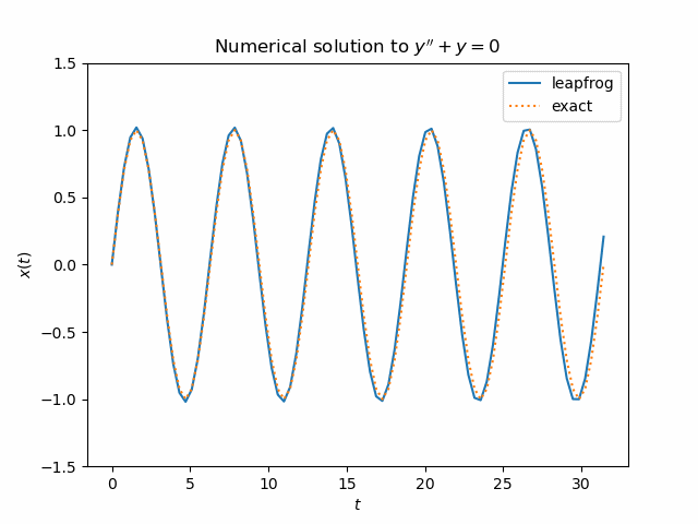
Here’s a plot of the solution over five periods.

There’s a lot more I hope to say about the leapfrog integrator and related methods in future posts.

NASA’s favorite ODE solver

Posted on 16 June 2020 by John

NASA’s Orbital Flight Handbook, published in 1963, is a treasure trove of technical information, including a section comparing the strengths and weaknesses of several numerical methods for solving differential equations.

The winner was a predictor-corrector scheme known as Gauss-Jackson, a method I have not heard of outside of orbital mechanics, but one apparently particularly well suited to NASA’s needs.

The Gauss-Jackson second-sum method is strongly recommended for use in either Encke or Cowell [approaches to orbit modeling]. For comparable accuracy, it will allow step-sizes larger by factors of four or more than any of the forth order methods. … As compared with unsummed methods of comparable accuracy, the Gauss-Jackson method has the very important advantage that roundoff error growth is inhibited. … The Gauss-Jackson method is particularly suitable on orbits where infrequent changes in the step-size are necessary.

Here is a table summarizing the characteristics of each of the solvers.

Notice that Gauss-Jackson is the only method whose roundoff error accumulation is described as “excellent.”

A paper from 2004 [1] implies that the Gauss-Jackson method was still in use at NASA at the time of writing.

The Gauss-Jackson multi-step predictor-corrector method is widely used in numerical integration problems for astrodynamics and dynamical astronomy. The U.S. space surveillance centers have used an eighth-order Gauss-Jackson algorithm since the 1960s.

I could imagine a young hotshot explaining to NASA why they should use some other ODE solver, only to be told that the agency had already evaluated the alternatives half a century ago, and that the competitors didn’t have the same long-term accuracy.

ODE solver landscape

Posted on 12 June 2020 by John

Many methods for numerically solving ordinary differential equations are either Runge-Kutta methods or linear multistep methods. These methods can either be explicit or implicit.

The table below shows the four combinations of these categories and gives some examples of each.

$\begin{tabular}{|l|ll|} \hline & Runge-Kutta & Linear multistep\\ \hline Explicit & ERK & Adams-Bashforth\\ Implicit & (S)DIRK & Adams-Moulton, BDF\\ \hline \end{tabular}$

Runge-Kutta methods advance the solution of a differential equation one step at a time. That is, these methods approximate the solution at the next time step using only the solution at the current time step and the differential equation itself.

Linear multistep methods approximate the solution at the next time step using the computed solutions at the latest several time steps.

Explicit methods express the solution at the next time step as an explicit function of other information, not including the solution itself. The solution at the next time step appears on only one side of the equations.

Implicit methods express the solution at the next time step as a function of other information including the solution itself. The solution at the next time step appears on both sides of the equations. Additional work needs to be done to solve for the solution.

More on explicit vs implicit methods here.

In the table above, ERK stands for, not surprisingly, explicit Runge-Kutta methods. DIRK stands for diagonally implicit Runge-Kutta. SDIRK stands for singly diagonally implicit Runge-Kutta. BDF stands for backward difference formulas.

Numerical analysis