Moments of Tukey’s g-and-h distribution

John Tukey developed his so-called g-and-h distribution to be very flexible, having a wide variety of possible values of skewness and kurtosis. Although the reason for the distribution’s existence is its range of possible skewness and values, calculating the skewness and kurtosis of the distribution is not simple.

Definition

Let φ be the function of one variable and four parameters defined by

\varphi(x; a, b, g, h) = a + b\left( \frac{\exp(gx) - 1}{g} \right) \exp(hx^2/2)

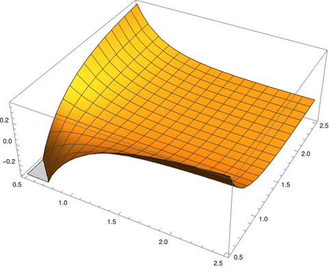
A random variable Y has a g-and-h distribution if it has the same distribution as φ(Z; a, b, g, h) where Z is a standard normal random variable. Said another way, if Y has a g-and-h distribution then the transformation φ−1 makes the data normal.

The a and b parameters are for location and scale. The name of the distribution comes from the parameters g and h that control skewness and kurtosis respectively.

The transformation φ is invertible but φ−1 does not have a closed-form; φ−1 must be computed numerically. It follows that the density function for Y does not have a closed form either.

Special cases

The g distribution is the g-and-h distribution with h = 0. It generalizes the log normal distribution.

The limit of the g-and-h distribution as g does to 0 is the h distribution.

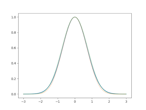
If g and h are both zero we get the normal distribution.

Calculating skewness and kurtosis

The following method of computing the moments of Y comes from [1].

Define f by

f(g, h, i) = \frac{1}{g^i\sqrt{1 - ih}} \sum_{r=0}^i \binom{i}{r} \exp\left(\frac{((i-r)g)^2}{2(1-ih)}\right)

Then the raw moments of Y are given by

\text{E} \, Y^m = \sum_{i=0}^m \binom{m}{i} a^{m-i}b^i f(g,h,i)

Skewness is the 3rd centralized moment and kurtosis is the 4th centralized moment. Equations for finding centralized moments from raw moments are given here.

Related posts

[1] James B. McDonald and Patrick Turley. Distributional Characteristics: Just a Few More Moments. The American Statistician, Vol. 65, No. 2 (May 2011), pp. 96–103

Symmetric functions and U-statistics

A symmetric function is a function whose value is unchanged under every permutation of its arguments. The previous post showed how three symmetric functions of the sides of a triangle

  • a + b + c
  • ab + bc + ac
  • abc

are related to the perimeter, inner radius, and outer radius. It also mentioned that the coefficients of a cubic equation are symmetric functions of its roots.

This post looks briefly at symmetric functions in the context of statistics.

Let h be a symmetric function of r variables and suppose we have a set S of n numbers where nr. If we average h over all subsets of size r drawn from S then the result is another symmetric function, called a U-statistic. The “U” stands for unbiased.

If h(x) = x then the corresponding U-statistic is the sample mean.

If h(x, y) = (xy)²/2 then the corresponding U-function is the sample variance. Note that this is the sample variance, not the population variance. You could see this as a justification for why sample variance as an n − 1 in the denominator while the corresponding term for population variance has an n.

Here is some Python code that demonstrates that the average of (xy)²/2 over all pairs in a sample is indeed the sample variance.

    import numpy as np
    from itertools import combinations

    def var(xs):
        n = len(xs)
        bin = n*(n-1)/2    
        h = lambda x, y: (x - y)**2/2
        return sum(h(*c) for c in combinations(xs, 2)) / bin

    xs = np.array([2, 3, 5, 7, 11])
    print(np.var(xs, ddof=1))
    print(var(xs))

Note the ddof term that causes NumPy to compute the sample variance rather than the population variance.

Many statistics can be formulated as U-statistics, and so numerous properties of such statistics are corollaries general results about U-statistics. For example U-statistics are asymptotically normal, and so sample variance is asymptotically normal.

Best line to fit three points

Suppose you want to fit a line to three data points. If no line passes exactly through your points, what’s the best compromise you could make?

minmax line for three points

Chebyshev suggested the best thing to do is find the minmax line, the line that minimizes the maximum error. That is, for each candidate line, find the vertical distance from each point to the line, and take the largest of these three distances as the measure of how well the line fits. The best line is the that minimizes this measure.

Note that this is not the same line you would get if you did a linear regression. Customary linear regression minimizes the average squared vertical distance from each point to the line. There are reasons this is the standard approach when you have at least a moderate amount of data, but when you only have three data points, it makes sense to use the minmax approach.

We can say several things about the minmax line. For one thing, there exists such a line and it is unique. Also, the vertical distance from each data point to the line will be the same. Either two points will be over the line and one under, or two will be under and one over.

Suppose your three points are (x1, y1), (x2, y2), and (x3, y3), with x1 < x2 < x3. Then the slope will be

m = \frac{y_3 - y_1}{x_3 - x_1}

and the intercept will be

b = \frac{y_1 (x_2+x_3)+y_2 (x_3-x_1) -y_3 (x_1+x_2)}{2 (x_3-x_1)}

I made an online calculator to find the best line for three points.

Cosine power approximation to Gaussian density


Years ago I wrote about how you can make a decent approximation to the Gaussian density by shifting and scaling the cosine function. This observation dates back at least as far as 1961.

Turns out you can do even better by raising the cosine term to a power. Not only can you get a good approximation, you can get an upper and lower bound of the same form.

In [1] the authors prove the following. For −π/2 < x < π/2,

\left( \frac{1 + \cos x}{2}\right)^a \leq \exp(-x^2) \leq \left( \frac{1 + \cos x}{2}\right)^b

and

\left( \frac{2 + \cos x}{3}\right)^c \leq \exp(-x^2) \leq \left( \frac{2 + \cos x}{3}\right)^d

with the best possible constants

\begin{align*} a &= 4 \\ b &= (\pi/2)^2/\log(2) \approx 3.559707\\ c &= (\pi/2)^2 / \log(3/2) \approx 6.08536\\ d &= 6 \end{align*}

When the authors say “best” they mean best with respect to L2 norm, i.e. best the the least-squares sense.

The graph at the top of the page plots exp(−x²) as solid blue line, the first upper bound as a dotted green line, and the first lower bound as a dotted orange line. The blue and green lines blend into a single bluish-green line. You can barely see the orange line separate from the others. The curves are difficult to distinguish visually, which is the point.

The second pair of upper and lower bounds are even better. Here’s a plot of the errors for the second pair of bounds.

gaps in bounds

Note that the theorem is stated for the interval [−π/2, π/2], but the plot covers a wider range in order to show that the errors are still small outside the interval. Outside the specified interval, the lower bound error becomes positive, i.e. the lower bound is no longer a lower bound, though it’s still a good approximation.

[1] Yogesh J. Bagul and Christophe Chesneau. Some sharp circular and hyperbolic bounds of exp(−x²) with applications. Applicable Analysis and Discrete Mathematics, Vol. 14, No. 1 (April 2020), pp. 239–254

Three advantages of non-AI models

It’s hard to imagine doing anything like Midjourney’s image generation without neural networks. The same is true of ChatGPT’s text generation. But a lot of business tasks do not require AI, and in fact would be better off not using AI. Three reasons why:

  1. Statistical models are easier to interpret. When a model has a dozen parameters, you can inspect each one. When a model has a billion parameters, not so much.
  2. Statistical models are more robust. Neural networks perform well on average, but fail in bizarre ways, and there is no way to explore all the possible edge cases. The edge cases of a statistical model can be enumerated, examined, and mitigated.
  3. Statistical models are not subject to legislation hastily written in response to recent improvements in AI. The chances that such legislation will have unintended consequences are roughly 100%.

Eccentricity of bivariate normal level sets

Suppose you have a bivariate normal distribution with correlation ρ where

f(x,y) = \frac{1}{2\pi \sqrt{1-\rho^2}} \exp\left(-\frac{x^2 - 2\rho xy + y^2}{2(1-\rho^2)} \right)

Then the level sets of the density function are ellipses, and the eccentricity e of the ellipses is related to the correlation ρ by

\begin{align*} \rho &= \pm \frac{e^2}{2 - e^2} \\ e &= \sqrt{\frac{2|\rho|}{1 + |\rho|} } \end{align*

Plots

For example, suppose ρ = 0.8.

Here’s a plot of the density function f(x, y).

And here is a plot of the contours, the level sets obtained by slicing the plot of the density horizontally.

Eccentricity and aspect ratio

The equation above says that since ρ = 0.8 the eccentricity e should be √(1.6/1.8) = 0.9428.

As I’ve written about several times, eccentricity is a little hard to interpret. It’s a number between 0 and 1, with 0 being a circle and 1 being a degenerate ellipse collapsed to a line segment. Since 0.9428 is closer to 1 than to 0, you might think that an ellipse with such a large value of e is very far from circular. But this is not the case.

Eccentric literally means off-center. Eccentricity measures how far off-center the foci of an ellipse are. This is related to how round or thin an ellipse is, but only indirectly. It is true that such a large value of e means that the foci are close to the ends of the ellipse. In fact, the foci are located at 94.28% of the distance from the center to the end of the semimajor axes. But the aspect ratio is more moderate.

It’s easier to imagine the shape of an ellipse from the aspect ratio than from the eccentricity. Aspect ratio r is related to eccentricity e by

r = \sqrt{1-e^2}

Using the expression above for eccentricity e as a function of correlation ρ we have

r = \sqrt{\frac{1 - |\rho|}{1 + |\rho|}}

This says our aspect ratio should be 1/3. So although our ellipse is highly eccentric—the foci are near the ends—it isn’t extraordinarily thin. It’s three times longer than it is wide, which matches the contour plot above.

Related posts

Bounds on the incomplete beta function (beta CDF)

The incomplete beta function is defined by

B(x, y, z) = \int_0^z t^{x-1} (1-t)^{y-1} \, dx

It is called incomplete because the limit of integration doesn’t necessarily run all the way up to 1. When z = 1 the incomplete beta function is simply the beta function

B(x, y) = B(x, y, 1)

discussed in the previous post [1].

The incomplete beta function is proportional to the CDF of a beta random variable, and the proportionality constant is 1/B(x, y). That is, if X is a beta(a, b) random variable, then

\text{Prob}(X \leq x) = \frac{B(a, b, x)}{B(a, b)}

The right-hand side of the equation above is often called the regularized incomplete beta function. This is what an analyst would call it. A statistician would call it the beta distribution function.

The previous post gave simple bounds on the (complete) beta function. This post gives bounds on the incomplete beta function. These bounds are more complicated but also more useful. The incomplete beta function is more difficult to work with than the beta function, and so upper and lower bounds are more appreciated.

One application of these bounds would be to speed up software that evaluates beta probabilities. If you only need to know whether a probability is above or below some threshold, you could first compute an upper or lower bound. Maybe computing the exact probability is unnecessary because you can decide from your bounds whether the probability is above or below your threshold. If not, then you compute the exact probability. This is less work if your bounds are usually sufficient, and more work if they’re usually not. In the former case this could result in a significant speed up because the incomplete beta function is relatively expensive to evaluate.

Cerone, cited in the previous post, gives two lower bounds, L1 and L2, and two upper bounds, U1 and U2, for B(x, y, z). Therefore the maximum of L1 and L2 is a lower bound and the minimum of U1 and U2 is an upper bound. The bounds are complicated, but easier to work with than the incomplete beta function.

\begin{align*} L_1 &= \frac{z^{x-1}}{y} \left[ \left(1 - z + \frac{z}{x} \right)^y - (1-z)^y \right] \\ U_1 &= \frac{z^{x-1}}{y} \left[ 1 - \left(1 - \frac{z}{x}\right)^y\right] \\ L_2 &= \frac{\lambda(z)^x}{x} + (1-z)^{y-1}\, \frac{z^x - \lambda(z)^x}{x} \\ U_2 &= (1-z)^{y-1} \frac{\left( x - \lambda(z) \right)^x}{x} + \frac{z^x - \left(z - \lambda(z)\right)^x}{x} \\ \end{align*}

where

\lambda(z) = \frac{1 - (1-z)[1 - z(1-y)]}{y\left[1-(1-z)^{y-1}\right]}

Related posts

[1] Incidentally, Mathematica overloads the Beta function just as we overload B. Mathematica’s Beta[x, y] corresponds to our B(x, y), but the three-argument version of Beta, the incomplete beta function, puts the limit of integration z first. That is, our B(x, y, z) corresponds to Beta[z, x, y] in Mathematica.

Upper and lower bounds on the beta function

The beta function B(x, y) is defined by

B(x, y) = \int_0^1 t^{x-1} (1-t)^{y-1}\, dt

and is the normalizing constant for the beta probability distribution. It is related to the gamma function via

B(x, y) = \frac{\Gamma(x)\,\Gamma(y)}{\Gamma(x+y)}

The beta function comes up often in applications. It can be challenging to work with, however, and so estimates for the function are welcome.

The function 1/xy gives simple approximation and upper bound for B(x, y). Alzer [1] proved that when x > 1 and y > 1

0 \leq \frac{1}{xy} - B(x,y) \leq b

where the constant b is defined by

b = \max_{x\geq1}\left( \frac{1}{x^2} - \frac{\Gamma(x)^2}{\Gamma(2x)} \right) = 0.08731\ldots

Cerone [2] gives a different bound which varies with x and y and is usually better than Alzer’s bound. For x and y greater than 1, Cerone shows

0 \leq \frac{1}{xy} - B(x,y) \leq C(x) C(y) \leq b'

where

C(x) = \frac{x-1}{x\sqrt{2x-1}}

and

C(x) = \frac{x-1}{x\sqrt{2x-1}}

Cerone’s bound is slightly larger in the worst case, near x = y = (3 + √5)/2, but is smaller in general.

The difference between B(x, y) and 1/xy is largest when x or y is small. We can visualize this with the Mathematica command

    Plot3D[Beta[x, y] - 1/(x y), {x, 0.5, 2.5}, {y, 0.5, 2.5}]

which produces the following plot.

The plot dips down in the corner where x and y are near 0.5 and curls upward on the edges where one of the variables is near 0.5 and the other is not.

Let’s look at B(x, y) and 1/xy at along a diagonal slice (3t, 4t).

This suggests that approximating B(x, y) with 1/xy works best when the arguments are either small or large, with the maximum difference being when the arguments are moderate-sized. In the plot we see B(3, 4) is not particularly close to 1/12.

Next lets look at 1/xyB(x, y) along the same diagonal slice.

This shows that the error bound C(x) C(y) is not too tight, but better than the constant bound except near the maximum of 1/xyB(x, y).

Related posts

[1] H. Alzer. Monotonicity properties of the Hurwitz zeta function. Canadian Mathematical Bulletin 48 (2005), 333–339.

[2] P. Cerone. Special functions: approximations and bounds. Applicable Analysis and Discrete Mathematics, 2007, Vol. 1, No. 1, pp. 72–91

Beta inequalities and cross ratios

When I worked at MD Anderson Cancer Center, we spent a lot of compute cycles evaluating the function g(a, b, c, d), defined as the probability that a sample from a beta(a, b) random variable is larger than a sample from a beta(c, d) random variable. This function was often in the inner loop of simulations that ran for hours or even days.

I developed ways to evaluate this function more efficiently because it was a bottleneck. Along the way I found a new symmetry. W. R. Thompson had studied what I call the function g back in 1933 and reported two symmetries:

g(a, b, c, d) = 1 − g(c, d, a, b)

and

g(a, b, c, d) = g(d, c, b, a).

I found that

g(a, b, c, d) = g(d, b, c, a)

as well. See a proof here.

You can conclude from these rules that

  1. g(a, b, c, d) = g(d, c, b, a) = g(d, b, c, a) = g(a, c, b, d)
  2. g(a, b, c, d) = 1 − g(c, d, a, b)

I was just looking at a book that mentioned the symmetries of the cross ratio which I will denote

r(a, b, c, d) = (ac)(b d) / (bc)(ad).

Here is Theorem 4.2 from [1] written in my notation.

Let a, b, c, d be four points on a projective line with cross ratio r(a, b, c, d) = λ. Then we have

    1. r(a, b, c, d) = r(b, a, d, c) = r(c, d, a, b) = r(d, c, b, a).
    2. r(a, b, d, c) = 1/λ
    3. r(a, c, b, d) = 1 − λ
    4. the values for the remaining permutations are consequences of these three basic rules.

This looks awfully familiar. Rules 1 and 3 for cross ratios correspond to rules 1 and 2 for beta inequalities, though not in the same order. Both g and r are invariant under reversing their arguments, but are otherwise invariant under different permutations of the arguments.

Both g and r take on 6 distinct values, taking on each 4 times. I feel like there is some deeper connection here but I can’t see it. Maybe I’ll come back to this later when I have the time to explore it. If you see something, please leave a comment.

There is no rule for beta inequalities analogous to rule 2 for cross ratios, at least not that I know of. I don’t know of any connection between g(a, b, c, d) and g(a, b, d, c).

Update: There cannot be a function h such that g(a, b, d, c) is a function of g(a, b, c, d) alone because I found parameters that lead to the same value of the latter but different values of the former. If there is a relation between g(a, b, c, d) and g(a, b, d, c) and it must involve the parameters and not just the value of g.

[1] Jürgen Richter-Gebert. Perspectives on Projective Geometry: A Guided Tour Through Real and Complex Geometry. Springer 2011.


Collecting a large number of coupons

This post is an addendum to the recent post Reviewing a thousand things. We’re going to look again at the coupon collector problem, randomly sampling a set of N things with replacement until we’ve collected one of everything.

As noted before, for large N the expected number of draws before you’ve seen everything at least once is approximately

N( log(N) + γ )

where γ is Euler’s constant.

A stronger result using a Chernoff bound says that for any constant c, the probability that the number of draws exceeds

N( log(N) + c )

approaches

1 − exp( − exp(−c))

as N increases. See [1].

I said in the earlier post that if you were reviewing a thousand things by sampling flash cards with replacement, there’s a 96% chance that after drawing 10,000 cards you would have seen everything. We could arrive at this result using the theorem above.

If N = 1,000 and we want N( log(N) + c ) to equal 10,000, we set c = 3.092. Then we find

1 − exp( − exp(−c) ) = 0.0444

which is consistent with saying there’s a 96% chance of having seen everything, 95.56% if you want to be more precise.


[1] Michael Mitzenmacher and Eli Upfal. Probability and Computing: Randomized Algorithms and Probabilistic Analysis. Cambridge University Press, 2005.