Powers of 3 + √2

Yesterday’s post looked at the distribution of powers of x mod 1. For almost all x > 1 the distribution is uniform in the limit. But there are exceptions, and the post raised the question of whether 3 + √2 is an exception.

A plot made it look like 3 + √2 is an exception, but that turned out to be a numerical problem.

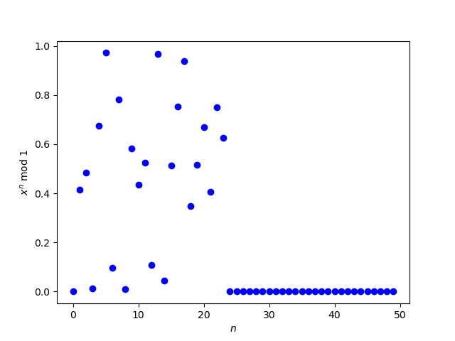
A higher precision calculation showed that the zeros on the right end of the plot were erroneous.

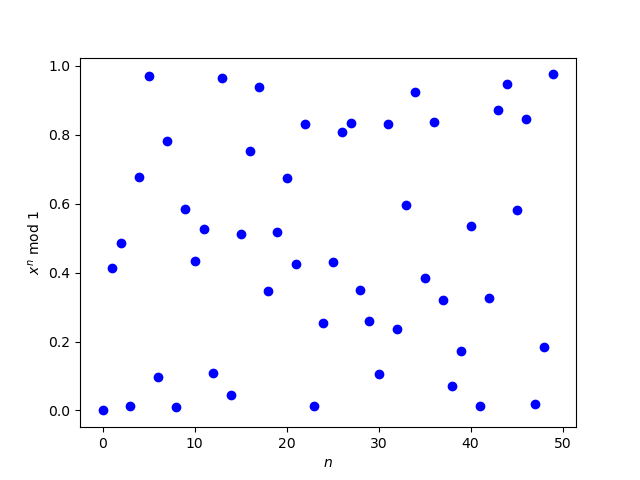
So this raises the question of how to calculate (3 + √2)n accurately for large n. The way I created the second plot was to use bc to numerically calculate the powers of 3 + √2. In this post, I’ll look at using Mathematica to calculate the powers symbolically.

For all positive integers n,

(3 + √2)n = an + bn√2

where an and bn are positive integers. We want to compute the a and b values.

If you ask Mathematica to compute (3 + √2)n it will simply echo the expression. But if you use the Expand function it will give you want you want. For example

    Expand[(3 + Sqrt[2])^10]

returns

    1404491 + 993054 √2

We can use the Coefficient function to split a + b √2 into a and b.

    parts[n_] := 
        Module[{x = (3 + Sqrt[2])^n}, 
            {Coefficient[x, Sqrt[2], 0], Coefficient[x, Sqrt[2], 1]}]

Now parts[10] returns the pair {1404491, 993054}.

Here’s something interesting. If we set

(3 + √2)n = an + bn√2

as above, then the two halves of the expression on the right are asymptotically equal. That is, as n goes to infinity, the ratio

anbn√2

converges to 1.

We can see this by defining

    ratio[n_] := 
        Module[ {a = Part[ parts[n], 1], b = Part[parts[n], 2]}, 
        N[a / (b Sqrt[2])]]

and evaluating ratio at increasing values of n. ratio[12] returns 1.00001 and ratio[13] returns 1, not that the ratio is exactly 1, but it is as close to 1 as a floating point number can represent.

This seems to be true more generally, as we can investigate with the following function.

    ratio2[p_, q_, r_, n_] := 
        Module[{x = (p + q Sqrt[r])^n}, 
            N[Coefficient[x, Sqrt[r], 0]/(Coefficient[x, Sqrt[r], 1] Sqrt[r])]]

When r is a prime and

(p + q√r)n = an + bnr

then it seems that the ratio an / bnr converges to 1 as n goes to infinity. For example, ratio2[3, 5, 11, 40] returns 1, meaning that the two halves of the expression for (3 + 5√11)n are asymptotically equal.

I don’t know whether the suggested result is true, or how to prove it if it is true. Feels like a result from algebraic number theory, which is not something I know much about.

Update: An anonymous person on X suggested a clever and simple proof. Observe that

\begin{align*} a_n &= \frac{(3+\sqrt{2})^n + (3-\sqrt{2})^n}{2} \\ b_n\sqrt{2} &= \frac{(3 + \sqrt{2})^n - (3-\sqrt{2})^n}{2} \end{align*}

In this form it’s clear that the ratio an / bn √2 converges to 1, and the proof can be generalized to cover more.

Multiples and powers mod 1

For a positive real number x, the expression x mod 1 means the fractional part of x:

x mod 1 = x − ⌊ x ⌋.

This post will look at the distributions of nx mod 1 and xn mod 1 for n = 1, 2, 3, ….

The distribution of nx mod 1 is easy to classify. If x is rational then nx will cycle through a finite number of values in the interval [0, 1]. If x is irrational then nx will be uniformly distributed in the interval.

The distribution of xn mod 1 is more subtle. We have three basic facts.

  1. If 0 ≤ x < 1, then xn → 0 as n → ∞.
  2. If x = 1 then xn = 1 for all n.
  3. For almost all x > 1 the sequence xn mod 1 is uniformly distributed. But for some values of x it is not, and there’s no known classification for these exceptional values of x.

The rest of the post will focus on the third fact.

Suppose x = √2. Then for all even n, xn mod 1 = 0. The sequence isn’t uniformly distributed in [0, 1] because half the sequence is piled up at 0.

For another example, let’s look at powers of the golden ratio φ = (1 + √5)/2. For even values of n the sequence φn converges to 1, and for odd values of n it converges to 0. You can find a proof here.

At one time it was not known whether xn mod 1 is uniformly distributed for x = 3 + √2.  (See HAKMEM, item 32.) I don’t know whether this is still unknown. Let’s see what we can tell from a plot.

Apparently sometime around n = 25 the sequence suddenly converges to 0. That looks awfully suspicious. Let’s calculate x25 using bc.

    $ echo '(3 + sqrt(2))^25' | bc -l
    13223107213151867.43024035874391918714

This says x25 mod 1 should be around 0.43, not near 0. The reason we’re seeing all zeros is that all the bits in the significand are being used to store the integer part and none are left over for the fractional part. A standard floating point number has 53 bits of significand and

(3 + √2)25 > 253.

For more details, see Anatomy of a floating point number.

Now let’s see what happens when we calculate xn mod 1 correctly using bc. Here’s the revised plot.

Is this uniformly distributed? Well, it’s not obviously not uniformly distributed. But we can’t tell by looking at a plot because uniform distribution is an asymptotic property.

We didn’t give the definition of a uniformly distributed sequence until now because an intuitive understanding of the term was sufficient. Now we should be more precise.

Given a set E, a sequence ω, and an integer N, define A(E, ω, N) to be the number of elements in the first N elements of the sequence ω that fall inside E. We say ω is uniformly distributed mod 1 if for every 0 ≤ ab ≤ 1,

limN → ∞ A([a, b), ω, N) / N = ba.

That is, the relative port of points that fall in an interval is equal to the length of the interval.

Now let’s go back to the example x = √2. We know that the powers of this value of x are not uniformly distributed mod 1. But we also said that for almost all x > 1 the powers of x are uniformly distributed. That means every tiny little interval around √2 contains a number y such that the powers of y are uniformly distributed mod 1. Now if y is very close to √2 and we plot the first few values of yn mod 1 then half of the values will be near 0. The sequence will not look uniformly distributed, though it is uniformly distributed in the limit.

Evaluating and lowering AI hallucination cost

AI models hallucinate, and always will [1]. In some sense this is nothing new: everything has an error rate. But what is new is the nature of AI errors. The output of an AI is plausible by construction [2], and so errors can look reasonable even when they’re wrong. For example, if you ask for the capital city of Illinois, an AI might err by saying Chicago, but it wouldn’t say Seattle.

You need to decide two things when evaluating whether to use an AI for a task: the cost of errors and the cost of validation.

Cost of error on horizontal axis, cost of validation on vertical axis

Image generation is an ideal task for AIs because the consequences of an error are usually low. And validation is almost effortless: if an image looks OK, it’s OK. So imagine generation is in the bottom left corner of the image above.

Text-to-speech is a little more interesting to evaluate. The consequences of an error depend on user expectations. Someone may be mildly annoyed when a computer makes an error reading an email out loud, but the same person may angry if he thought he was talking to a human and discovers he’s been talking to a machine.

Validating text-to-speech requires a human to listen to the audio. This doesn’t require much effort, though the cost might be too much in some contexts. (I’m in the middle of an AI-narrated book and wondering why the producer didn’t go to the effort of fixing the pronunciation errors. The print version of the book has high production quality, but not as much effort went into the audio.) So I’d say text-to-speech is somewhere in the bottom half of the graph, but the horizontal location depends on expectations.

Code generation could be anywhere on the graph, depending on who is generating the code and what the code is being used for. If an experienced programmer is asking AI to generate code that in principle he could have written, then it should be fairly easy to find and fix errors. But it’s not a good idea for a non-programmer to generate code for a safety-critical system.

Mitigating risks and costs

The place you don’t want to be is up and to the right: errors are consequential and validation is expensive. If that’s where your problem lies, then you want to either mitigate the consequences of errors or reduce the cost of validation.

This is something my consultancy helps clients with. We find ways to identify errors and to mitigate the impact of inevitable errors that slip through.

If you’d like help moving down and to the left, lowering the cost of errors and the cost of validation, let’s set up a meeting to discuss how we can help.

LET’S TALK

[1] LLMs have billions of parameters, pushing a trillion. But as large as the parameter space is, the space of potential prompts is far larger, and so the parameters do not contain enough information to respond completely accurately to every possible prompt.

[2] LLMs predict the word that is likely to come next given the words produced so far. In that sense, the output is always reasonable. If an output does not appear reasonable to a human, it is because the human has more context.

A Continental Divide for Newton’s Method

Newton’s method is a simple and efficient method for finding the roots of equations, provided you start close enough to the root. But determining the set of starting points that converge to a given root, or converge at all, can be very complicated.

In one case it is easy to completely classify where points converge. Suppose you have a quadratic polynomial p(x) with distinct roots a and b in the complex plane. The line perpendicular to the line between a and b is a sort of continental divide, splitting the plane into two watersheds. If you start Newton’s method at any point on a root’s side of the line, it will converge to that root.

To illustrate this, we will set a = 7 + 14i and b = 20 + 25i, and use Newton’s method to find the roots of

p(z) = (z − a)(z − b).

You can start far from the root and still converge, which isn’t typical but is the case for quadratic polynomials.

And the point you’ll converge to is determined by which side of the continental divide you start on. For example, the following code shows that if you start at 1000 + 2000i you will converge to 20 + 25i.

a = 7 + 14j
b = 20 + 25j

p      = lambda z: (z - a)*(z - b)
pprime = lambda z: (z - a) + (z - b)
newton = lambda z: z - p(z)/pprime(z)

z = 1000 + 2000j
for _ in range(12):
    z = newton(z)
    print(z)

If you’re not familiar with Python, note that it uses j for the imaginary unit. Here’s why.

Things are more complicated if you start Newton’s method exactly on the line dividing the two watersheds. The method will not converge. There is a dense set of starting points on the line that will cycle through a finite number of points. And there is a dense set of points that lead to division by zero. (See HAKMEM, item 3.)

Related posts

Experiences with Nvidia

Our team started working within Nvidia in early 2009 at the beginning of the ORNL Titan project. Our Nvidia contacts dealt with applications, libraries, programming environment and performance optimization. First impressions were that their technical stance on issues was very reasonable. One obscure example: in a C++ CUDA kernel were you allowed to use “enums,” and the answer would be, of course, yes, we would allow that. This was unlike some other companies that might have odd and cumbersome programming restrictions in their parallel programming models (though by now this has become a harder problem for Nvidia since there are so many software products a user might want to interoperate).

Another example, with a colleague at Nvidia on the C++ standards committee, to whom I mentioned, it might be too early to lock this certain feature design into the standard since hardware designs are still rapidly changing. His response was, Oh, yes, we think exactly the same thing. So in short, their software judgments and decisions generally seem to be well thought out, reasonable and well informed. It sounds simple, but it is amazing how many companies have gotten this wrong.

Nvidia has made good strategic decisions. In the 2013 time frame, Intel was becoming a competitive threat with the Xeon Phi processor. Intel was several times larger than Nvidia with huge market dominance. In response, Nvidia formed a partnership with IBM–itself several times larger than Intel at the time. This came to fruition in the ORNL Summit system in 2018. In the meantime, the Xeon Phi’s OpenMP programming model, though standards-based, turned out to be difficult to write optimized code for, and Nvidia CUDA captured market share dominance of accelerated user software. Intel eventually dropped the Xeon Phi product line.

In the early 2000s, Nvidia went all-in on CUDA. I’ve heard some project teams say they would never use CUDA, because it is nonstandard and too low-level. Many have turned back on this decision. Of course, it is often possible to write an abstraction layer on top of CUDA to make it easier to use and maintain. Also newer programming models like Kokkos can be helpful.

Nvidia also made a prescient decision early to bet big on AI. A little later they decided to go all in on developing a huge number of software libraries is to enable access to many new markets. A huge moat. AMD is trying hard to improve their software processes and catch up.

On the downside, Nvidia high prices are upsetting to many, from gamers to buyers of the world’s largest HPC systems. Competition from AMD and others is a good thing.

And Nvidia marketing speak is sometimes confusing. A comparison was once made claiming that a four GPU system was more powerful than one of the world’s top CPU-only supercomputers on a very specific science problem. I’d like to see the details of that comparison. Also, different figures are being given on how long it took to stand up xAI’s Colossus supercomputer, from 19 days to 122 days. One has to dig a little to find out what these figures mean. Also it was widely reported last year that the GB200 NVL72 GPU was “30 times faster” than H100, but this only refers to certain operations, not key performance measures like flops per watt.

Those are my takes. For more perspectives, see Tae Kim’s excellent book, The Nvidia Way, or this interview.

Thoughts on Nvidia? Please leave in the comments.


Legendre polynomials

The previous post mentioned Legendre polynomials. This post will give a brief introduction to these polynomials and a couple hints of how they are used in applications.

One way to define the Legendre polynomials is as follows.

  • P0(x) = 1
  • Pk are orthogonal on [−1, 1].
  • Pk(1) = 1 for all k ≥ 0.

The middle bullet point means

\int_{-1}^1 P_m(x) P_n(x) \, dx = 0

if mn. The requirement that each Pk is orthogonal to each of its predecessors determines Pk up to a constant, and the condition Pk(1) = 1 determines this constant.

Here’s a plot of the first few Legendre polynomials.

There’s an interesting pattern that appears in the white space of a graph like the one above when you plot a large number of Legendre polynomials. See this post.

The Legendre polynomial Pk(x) satisfies Legendre’s differential equation; that’s what motivated them.

(1 - x^2) y^{\prime\prime} -2x y^\prime + k(k+1)y = 0

This differential equation comes up in the context of spherical harmonics.

Next I’ll describe a geometric motivation for the Legendre polynomials. Suppose you have a triangle with one side of unit length and two longer sides of length r and y.

You can find y in terms of r by using the law of cosines:

y = \sqrt{1 - 2r \cos \theta + r^2}

But suppose you want to find 1/y in terms of a series in 1/r. (This may seem like an arbitrary problem, but it comes up in applications.) Then the Legendre polynomials give you the coefficients of the series.

\frac{1}{y} = \frac{P_0(\cos\theta)}{r} + \frac{P_1(\cos\theta)}{r^2} + \frac{P_2(\cos\theta)}{r^3} + \cdots

Source: Keith Oldham et al. An Atlas of Functions. 2nd edition.

Related posts

The biggest perturbation of satellite orbits

To first approximation, a satellite orbiting the earth moves in an elliptical orbit. That’s what would get from solving the two-body problem: two point masses orbiting their common center of mass, subject to no forces other than their gravitational attraction to each other.

But the earth is not a point mass. Neither is a satellite, though that’s much less important. The fact that the earth is not exactly a sphere but rather an oblate spheroid is the root cause of the J2 effect.

The J2 effect is the largest perturbation of a satellite orbit from a simple elliptical orbit, at least for satellites in low earth orbit (LEO) and medium earth orbit (MEO). The J2 effect is significant for satellites in higher orbits, though third body effects are larger.

Legendre showed that the gravitational potential of an axially symmetric planet is given by

V(r, \phi) = \frac{Gm}{r} \left( 1 - \sum_{k=2}^\infty J_k  \left( \frac{r_{eq}}{r}\right)^k P_k(\cos \phi) \right)

Here (r, φ) are spherical coordinates. There’s no θ term because we assume the planet, and hence its gravitational potential, is axially symmetric, i.e. independent of θ. The term req is the equatorial radius of the planet. The Pk are Legendre polynomials.

For a moderately oblate planet, like the one we live on, the J2 coefficient is much larger than the others, and neglecting the rest of the coefficients gives a good approximation [1].

Here are the first few coefficients for Earth [2].

\begin{align*} J_2 &= \phantom{-}0.00108263 \\ J_3 &= -0.00000254 \\ J_4 &= -0.00000161 \end{align*}

Note that J2 is three orders of magnitude smaller than 1, and so the J2 effect is small. And yet it matters a great deal. The longitude of the point at which a satellite crosses the equatorial plane may vary a few degrees per day. The rate of precession is approximately proportional to J2.

The value of J2 for Mars is about twice that of Earth (0.001960454). The largest J2 in our solar system is Neptune, which is about three times that of Earth (0.003411).

There are many factors left out of the assumptions of the two body problem. The J2 effect doesn’t account for everything that has been left out, but it’s the first refinement.

More orbital mechanics posts

More Legendre posts

[1] Legendre discovered/invented what we now call the Legendre polynomials in the course of calculating the gravitational potential above. I assume the convention of using J for the coefficients goes back to Legendre.

[2] Richard H. Battin. An Introduction to the Mathematics and Methods of Astrodynamics, Revised Edition, 1999.

Transmission Obstacles and Ellipsoids

Suppose you have a radio transmitter T and a receiver R with a clear line of sight between them. Some portion the signal received at R will come straight from T. But some portion will have bounced off some obstacle, such as the ground.

The reflected radio waves will take a longer path than the waves that traveled straight from T to R. The worst case for reception is when the waves traveling a longer path arrive half a period later, i.e. 180° out of phase, canceling out part of the signal that was received directly.

We’d like to describe the region of space that needs to be empty in order to eliminate destructive interference, i.e. signals 180° out of phase. Suppose T and R are a distance d apart and the wavelength of your signal is λ. An obstacle at a location P can cause signals to arrive exactly out of phase if the distance from T to P plus the distance from P to R is d + λ/2.

So we’re looking for the set of all points such that the sum of their distances to fixes points is a constant. This is the nails-and-string description of an ellipse, where the nails are a distance d apart and the string has length d + λ/2.

That would be a description of the region if we were limited to a plane, such as a plane perpendicular to the ground and containing the transmitter and receiver. But signals could reflect off an obstacle that’s outside this plane. So now we need to imagine being able to move the string in three dimensions. We still get all the points we’d get if we were restricted to a plane, but we also get their rotation about the axis running between T and R.

The region we’re describing is an ellipsoid, known as a Fresnel ellipsoid or Fresnel zone.

Suppose we choose our coordinates so that our transmitter T is located at (0, 0, h) and our receiver R is located at (d, 0, h). We imagine a string of length d + λ/2 with endpoints attached to T and R. We stretch the string so it consists of two straight segments. The set of all possible corners in the string traces out the Fresnel ellipsoid.

Greater delays

If reflected waves are delayed by exactly one period, they reinforce the portion of the signal that arrived directly. Signals delayed by an even multiple of a half-period cause constructive interference, but signals delayed by odd multiples of a half-period cause destructive interference. The odd multiples matter most because we’re more often looking to avoid destructive interference rather than seeking out opportunities for constructive interference.

If you repeat the exercise above with a string of length length d + λ you have another Fresnel ellipsoid. The foci remain the same, i.e. T and R, but this new ellipsoid is bigger since the string is longer. This ellipsoid represents locations where a signal reflected at that point will arrive one period later than a signal traveling straight. Obstacles on the surface of this ellipsoid cause constructive interference.

We can repeat this exercise for a string of length d + nλ/2, where odd values of n correspond to regions of destructive interference. This gives us a set of confocal ellipsoids known as the Fresnel ellipsoids.

Related posts

Zooming in on a fractalish plot

The exponential sum of the day page on my site draws an image every day by plugging the month, day, and year into a formula. Details here.

Today’s image looks almost solid blue in the middle.

The default plotting line width works well for most days. For example, see what the sum of the day will look line on July 1 this year. Making the line width six times thinner reveals more of the detail in the middle.

You can see even more detail in a PDF of the plot.