Integrating polynomials over a sphere or ball

Spheres and balls are examples of common words that take on a technical meaning in math, as I wrote about here. Recall the unit sphere in n dimensions is the set of points with distance 1 from the origin. The unit ball is the set of points of distance less than or equal to 1 from the origin. The sphere is the surface of the ball.

Integrating a polynomial in several variables over a ball or sphere is easy. For example, take the polynomial xy² + 5x²z² in three variables. The integral of the first term, xy², is zero. If any variable in a term has an odd exponent, then the integral of that term is zero by symmetry. The integral over half of the sphere (ball) will cancel out the integral over the opposite half of the sphere (ball). So we only need to be concerned with terms like 5x²z².

Now in n dimensions, suppose the exponents of x1, x2, …, xn are a1, a2, …, an respectively. If any of the a‘s are odd, the integral over the sphere or ball will be zero, so we assume all the a‘s are even. In that case the integral over the unit sphere is simply

2 B(b_1, b_2, \ldots, b_n)

where

B(b_1, b_2, \ldots, b_n) = \frac{\Gamma(b_1) \Gamma(b_2) \cdots \Gamma(b_n)}{ \Gamma(b_1 + b_2 + \cdots + b_n)}

is the multivariate beta function and for each i we define bi = (ai + 1)/2. When n = 2 then B is the (ordinary) beta function.

Note that the integral over the unit sphere doesn’t depend on the dimension of the sphere.

The integral over the unit ball is

\frac{2 B(b_1, b_2, \ldots, b_n)}{ a_1 + a_2 + \cdots + a_n + n}

which is proportional to the integral over the sphere, where the proportionality constant depends on the sum of the exponents (the original exponents, the a‘s, not the b‘s) and the dimension n.

Note that if we integrate the constant polynomial 1 over the unit sphere, we get the surface area of the unit sphere, and if we integrate it over the unit ball, we get the volume of the unit ball.

You can find a derivation for the integral results above in [1]. The proof is basically Liouville’s trick for integrating the normal distribution density, but backward. Instead of going from rectangular to polar coordinates, you introduce a normal density and go from polar to rectangular coordinates.

[1] Gerald B. Folland, How to Integrate a Polynomial over a Sphere. The American Mathematical Monthly, Vol. 108, No. 5 (May, 2001), pp. 446-448.

Bounding the 3rd moment by the 4th moment

For a random variable X, the kth moment of X is the expected value of Xk.

For any random variable X with 0 mean, or negative mean, there’s an inequality that bounds the 3rd moment, m3 in terms of the 4th moment, m4:

m_3 \leq \left(\frac{4}{27} \right )^{1/4} m_4^{3/4}

The following example shows that this bound is the best possible.

Define

u = (1 − √ 3)/√ 2
v = (1 + √ 3)/√ 2
p = (3 + √ 3) / 6

and suppose Xu with probability p and Xv with probability q = 1 − p. Then X has mean 0, and you can show that exact equality holds in the inequality above.

Here’s some Mathematica code to verify this claim.

    u = (1 - Sqrt[3])/Sqrt[2]
    v = (1 + Sqrt[3])/Sqrt[2]
    p = (Sqrt[3] + 1)/(2 Sqrt[3])
    q = 1 - p
    m3 = p u^3 + q v^3
    m4 = p u^4 + q v^4
    Simplify[ (4/27)^(1/4) m4^(3/4) / m3 ]

As hoped, the code returns 1.

Reference: Iosif Pinelis, Relations Between the First Four Moments, American Mathematical Monthly, Vol 122, No 5, pp 479-481.

Putting a brace under something in LaTeX

Here’s a useful LaTeX command that I learned about recently: \underbrace.

It does what it sounds like it does. It puts a brace under its argument.

I used this a few days ago in the post on the new prime record when I wanted to show that the record prime is written in hexadecimal as a 1 followed by a long string of Fs.

1\underbrace{\mbox{FFF \ldots FFF}}_\mbox{{\normalsize 9,308.229 F's}}

The code that produced is

1\underbrace{\mbox{FFF \ldots FFF}}_\mbox{{\normalsize 9,308.229 F's}}

The sizing is a little confusing. Without \normalsize the text under the brace would be as large as the text above.

Emacs features that use regular expressions

The syntax of regular expressions in Emacs is a little disappointing, but the ways you can use regular expressions in Emacs is impressive.

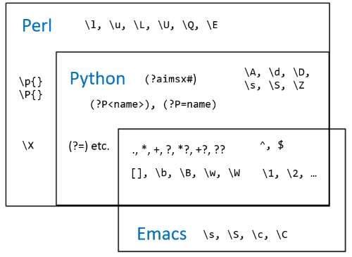
I’ve written before about the syntax of Emacs regular expressions. It’s a pretty conservative subset of the features you may be used to from other environments as summarized in the diagram below.

But there are many, many was to use regular expressions in Emacs. I did a quick search and found that about 15% of the pages in the massive Emacs manual contain at least one reference to regular expressions. Exhaustively listing the uses of regular expressions would not be practical or very interesting. Instead, I’ll highlight a few uses that I find helpful.

Searching and replacing

One of the most frequently used features in Emacs is incremental search. You can search forward or backward for a string, searching as you type, with the commands C-s (isearch-forward) and C-r (isearch-backward). The regular expression counterparts of these commands are C-M-s (isearch-forward-regexp) and C-M-r (isearch-backward-regexp).

Note that the regular expression commands add the Alt (meta) key to their string counterparts. Also, note that Emacs consistently refers to regular expressions as regexp and never, as far as I know, as regex. (Emacs relies heavily on conventions like this to keep the code base manageable.)

A common task in any editor is to search and replace text. In Emacs you can replace all occurrences of a regular expression with replace-regexp or interactively choose which instances to replace with query-replace-regexp.

Purging lines

You can delete all lines in a file that contain a given regular expression with flush-lines. You can also invert this command, specifying which lines not to delete with keep-lines.

Aligning code

One lesser-known but handy feature is align-regexp. This command will insert white space as needed so that all instances of a regular expression in a region align vertically. For example, if you have a sequence of assignment statements in a programming language you could have all the equal signs line up by using align-regexp with the regular expression consisting simply of an equal sign. Of course you could also align based on a much more complex pattern.

Although I imagine this feature is primarily used when editing source code, I imagine you could use it in other context such as aligning poetry or ASCII art diagrams.

Directory editing

The Emacs directory editor dired is something like the Windows File Explorer or the OSX Finder, but text-based. dired has many features that use regular expressions. Here are a few of the more common ones.

You can mark files based on the file names with % m (dired-mark-files-regexp) or based on the contents of the files with % g (dired-mark-files-containing-regexp). You can also mark files for deletion with % d (dired-flag-files-regexp).

Inside dired you can search across a specified set of files by typing A (dired-do-find-regexp), and you can interactively search and replace across a set of files by typing Q (dired-do-find-regexp-and-replace).

Miscellaneous

The help apropos command (C-h a) can take a string or a regular expression.

The command to search for available fonts (list-faces-display) can take a string or regular expression.

Interactive highlighting commands (highlight-regexp, unhighlight-regexp, highlight-lines-matching-regexp) take a regular expression argument.

You can use a regular expression to specify which buffers to close with kill-matching-buffers.

Maybe the largest class of uses for regular expressions in Emacs is configuration. Many customizations in Emacs, such as giving Emacs hints to determine the right editing mode for a file or how to recognize comments in different languages, use regular expressions as arguments.

Resources

You can find more posts on regular expressions and on Emacs by going to my technical notes page. Note that the outline at the top has links for regular expressions
and for Emacs.

For daily tips on regular expressions or Unix-native tools like Emacs, follow @RegexTip and @UnixToolTip on Twitter.

Easter eggs and yellow pigs

An Easter egg is a hidden feature, a kind of joke. The term was first used in video games but the idea is broader and older than that. For example, Alfred Hitchcock made a brief appearance in all his movies. And I recently heard that there’s a pineapple or reference to a pineapple in every episode of the television show Psych.

Michael Spivak put references to “yellow pig” in some of his books. I’ve heard that he put allusions to yellow pigs in all his books, but I don’t have all his books, and I haven’t been able to find yellow pigs in two of his books that I do own.

Spivak’s calculus text is dedicated to the memory of Y. P.

Dedicated to the Memory of Y. P.

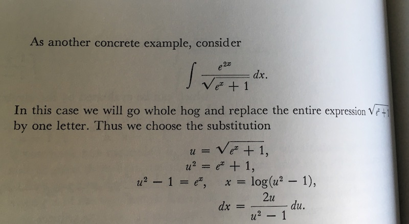
If you look up yellow pig in the index of the book, it will take you to a page that makes a passing reference to “whole hog.”

Spivak’s publishing company, Publish or Perish Press, originally used a pig as part of its logo.

Publish or Perish old logo

The website now has no logo. His most recent book, Physics for Mathematicians: Mechanics I, uses a different logo.

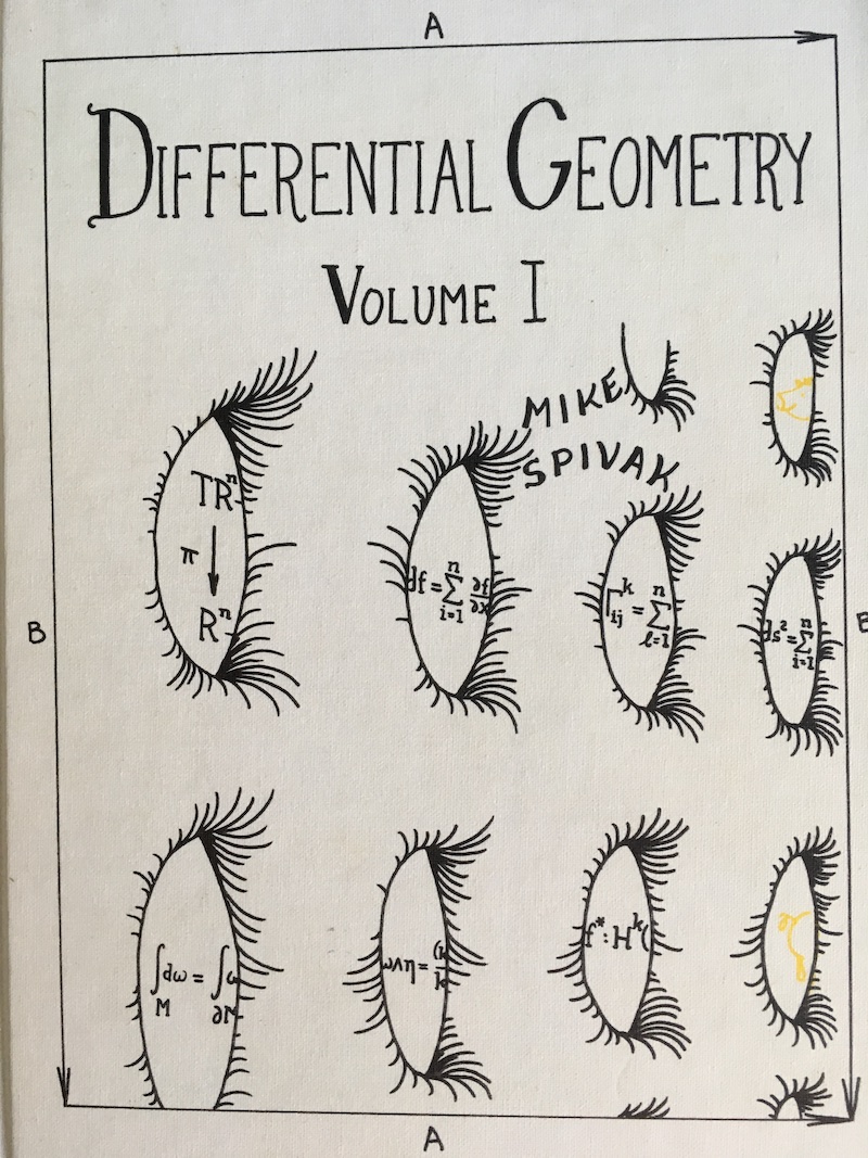
The cover of Spivak’s Differential Geometry, Volume 1, second edition, has two yellow drawings of a pig.

Cover of Spivak's Differential Geometry, Volume 1, second edition

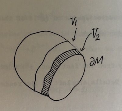
If you look up yellow pig in the index, it takes you to a page that doesn’t mention pigs, but does include a drawing that looks something like a ham.

Ham-like illustration from Spivak's Differential Geometry, volume 1

I do not see a reference to yellow pig in Spivak’s first book, Calculus on Manifolds. It was published by Benjamin Cummings. Maybe they would not allow Easter eggs, or maybe the idea of including Easter eggs didn’t occur to Spivak until he had his own publishing company. I also do not see a reference to yellow pigs in his recent Physics for Mathematicians book.

Big derivatives

Suppose you have a function of n variables f. The kth derivative of f is a kth order tensor [1] with nk components.

Not all those tensor components are unique. Assuming our function f is smooth, the order in which partial derivatives are taken doesn’t matter. It only matters which variables you differentiate with respect to and how many times.

There is a potentially unique component of the kth order derivative for every choice of k items (the variables you’re differentiating with respect to) from a set of n items (the variables) with replacement (because you can differentiate with respect to the same variable multiple times). Richard Stanley introduced the notation

\left( {n \choose k} \right)

for this quantity, and it turns out that

\left( {n \choose k} \right) = {n + k - 1 \choose k}

See Counting selections with replacement.

If n or k are large, this is a very large number. Suppose you have a function of n = 1,000 variables and you want to take the 5th derivative. The derivative has 1015 components, but “only” about 1013 distinct components. 8,416,958,750,200 to be exact. A floating point number (IEEE 754 double) takes up 8 bytes, so storing the distinct components would require 62,711 gigabytes. So you could store the distinct components if you had a thousand computers with 64 GB of RAM each.

An application that depends on high-order derivatives of functions of many variables has to exploit some structure, such as sparsity or symmetry, and not directly compute and store the derivatives.

By the way, if both are large, the approximate number of components estimated via Stirling’s approximation is

\sqrt{\frac{m+k}{2\pi m k}} \frac{(m+k)^{m+k}}{m^m k^k}

where mn − 1.

***

[1] The value of the function is a real number, a scalar, a 0th order tensor. The first derivative, the gradient, is a vector, a 1st order tensor. The second derivative, the Hessian, is a matrix, a 2nd order tensor. There aren’t more common names for tensors of order three and higher. You could think of a 3rd order tensor as a three dimensional box of numbers, a stack of matrices.

Are coffee and wine good for you or bad for you?

wine coffee

One study will say that coffee is good for you and then another will say it’s bad for you. Ditto with wine and many other things. So which is it: are these things good for you or bad for you?

Probably neither. That is, these things that are endlessly studied with contradictory conclusions must not have much of an effect, positive or negative, or else studies would be more definitive.

John Ioannidis puts this well in his recent interview on EconTalk:

John Ioannidis: … We have performed hundreds of thousands of studies trying to look whether single nutrients are associated with specific types of disease outcomes. And, you know, you see all these thousands of studies about coffee, and tea, and all kind of —

Russ Roberts: broccoli, red meat, wine, …

John Ioannidis: — things that you eat. And they are all over the place, and they are always in the news. And I think it is a complete waste. We should just decide that we are talking about very small effects. The noise is many orders of magnitude more than the signal. If there is a signal. Maybe there is no signal at all. So, why are we keep doing this? We should just pause, and abandon this type of design for this type of question.

Distribution of matches between two shuffled decks

Take two desks of cards and shuffle them. They can be standard 52-card decks, though the number of cards in the decks doesn’t matter as long as they’re the same and the decks are fairly large.

Now count the number of times the two desks match, i.e. how many times the same card is in the same position in both desks. The number of matches is random, and its distribution is approximately Poisson with mean 1. Let’s do a simulation and see how close the results come to the predicted outcome.

Here’s the Python code:

import numpy as np
from scipy.stats import poisson
import matplotlib.pyplot as plt

def count_zeros(x):
    return len(x[x==0])

num_reps = 10000
deck_size = 52

matches = np.zeros(deck_size+1, dtype=int)

# Simulation
for _ in range(num_reps):

    # Shuffle two decks
    a = np.random.permutation(deck_size)
    b = np.random.permutation(deck_size)

    # Count how often they match
    num_matches = count_zeros(a-b)
    matches[ num_matches ] += 1

# Cut off outputs too small to see
cutoff = 8

# Matches predicted by a Poisson distribution with mean 1.
predicted = [num_reps*poisson(1).pmf(i) for i in range(cutoff)]

# Plot results
x = np.arange(cutoff)
w = 0.3 # bar width
plt.bar(x, matches[0:cutoff], w)
plt.bar(x+w, predicted, w)
plt.legend(["actual", "predicted"])
plt.xlabel("matches")
plt.ylabel("frequency")
plt.savefig("shuffled_desk_matches.svg")
plt.show()

And here’s the output based on 10,000 simulations:

Plot showing good fit between predicted and actual

About 1/3 of the time, you get no matches, another 1/3 of the time you get one match, and the rest of the time you get more. More precisely, according to the Poisson model zero matches and one match are both have probability 1/e.

Magic squares as matrices

If you view a 3 × 3 magic square as a matrix and raise it to the third power, the result is also a magic square.

More generally, if you multiply an odd number of 3 × 3 magic squares together, the result is a magic square.

For example, here are three magic squares that appeared in my blog post on Spanish magic squares, and you can verify that their product is another magic square.

\left[ \begin{array}{ccc} 93 & 155 & 121 \\ 151 & 123 & 95 \\ 125 & 91 & 153 \\ \end{array} \right] \left[ \begin{array}{ccc} 12 & 21 & 15 \\ 19 & 16 & 13 \\ 17 & 11 & 20 \\ \end{array} \right] \left[ \begin{array}{ccc} 13 & 20 & 18 \\ 22 & 17 & 12 \\ 16 & 14 & 21 \\ \end{array} \right] = \left[ \begin{array}{ccc} 299622 & 301968 & 301722 \\ 303204 & 301104 & 299004 \\ 300486 & 300240 & 302586 \\ \end{array} \right]

Source: Martin Gardner, Some New Discoveries About 3 × 3 Magic Squares, Math Horizons, February 1998.

The same article conjectures that the results above are true for magic squares of any odd order. That was 20 years ago. Maybe the conjecture has been resolved by now. If you know, please leave a comment.

More magic square posts

GDPR and the right to be forgotten

George Bailey on the Bedford Falls bridge

General Data Protection Regulation

The European GDPR (General Data Protection Regulation) was adopted in 2016 and becomes enforceable in May of this year. Article 17 mandates a right to erasure, more commonly called the right to be forgotten.

A right to be forgotten is tricky. It’s not immediately clear what this means or to what extent it’s even possible. That’s for lawyers and courts to work out. I can’t comment on the legal interpretation of the regulation. There are laws that require companies to delete information and laws that require them to retain information, and no doubt there are debates on how to reconcile these.

Here I want to look at some of the logical and statistical issues that come out of privacy laws, not necessarily the GDPR in particular, that mandate that information be forgotten.

Challenges with a right to be forgotten

Suppose John Smith had participated in some database and a report showed that there were 5,000 diabetics in Smith’s geographic region. Smith asks to be removed from the database, and now a revised report shows that there are 4,999 diabetics in the region. What does that tell you about Smith? (For an elaboration on this example, see Big aggregate queries can still violate privacy.)

You might object that removing Smith from the database doesn’t really cause him to be forgotten if we retain the fact that he was removed from the database. We have to forget that he was forgotten, maybe like George Bailey in “It’s a Wonderful Life.” While the fictional George Bailey was able to see what life would have been like if he had never been born, our real-world John Smith doesn’t have that option. Truly forgetting anything in a world of ubiquitous databases may not be possible. It may require a cascade of changes that are illegal, impractical, or impossible.

Differential privacy

One way to address the challenges of erasure is though differential privacy. A report constructed via a differentially private system would not have released the exact number of diabetics in Smith’s region but rather some randomized version of the exact result. Ideally the amount of noise added to the true result is large enough to protect Smith’s privacy, but small enough that the result is useful to the person who wants to know the approximate number of diabetics in Smith’s region.

Differential privacy is both powerful and subtle. It gives a theoretically grounded way to quantify the privacy implications of someone’s participation or lack of participation in a database. But it comes with restrictions that may be hard to live with. For example, we cannot let someone ask the same question many times, or if we do, we must give the same answer each time. If the answers were generated afresh each time, one could average the results to remove the effect of the random noise.

But what if you want to let someone rerun reports, not because they’re trying to evade privacy protections, but because the world is changing and they periodically want to get an updated view of the world? That can be done, but it requires forethought. Before you release the first report, you must have a system in place that is intended to allow multiple queries over time.

Differential privacy applies to a process, not to a result. You can’t say “This is a differentially private report” but rather “This report is the result of a differentially private mechanism.” That mechanism has to be designed up front. You can design a mechanism to support a wide variety of queries, but this comes at a cost. You have to anticipate what these queries will be (maybe not specifically but at least some class that they fall in) and add sufficient randomness to support them all. In general, the more flexible you want your query system to be, the more randomness you will need to add, and so you face a privacy-utility trade-off.

Help with privacy compliance

If you’d like help with privacy law compliance, let’s talk. I help companies with statistical matters related to privacy, such as expert determination of de-identification (or pseudonymisation as it’s known in Europe). I am not an expert on the regulatory side of things, but I work in coordination with lawyers who are.