arctan( k tan(x) )

Posted on 18 November 2019 by John

I recently had to work with the function

f(x; k) = arctan( k tan(x) )

The semicolon between x and k is meant to imply that we’re thinking of x as the argument and k as a parameter.

This function is an example of the coming full circle theme I’ve written about several times. Here’s how a novice, a journeyman, and an expert might approach studying our function.

Novice: arctan( k tan(x) ) = kx.
Journeyman: You can’t do that!
Expert: arctan( k tan(x) ) ≈ kx for small x.

Novices often move symbols around without thinking about their meaning, and so someone might pull the k outside (why not?) and notice that arctan( tan(x) ) = x.

Someone with a budding mathematical conscience might conclude that since our function is nonlinear in x and in k that there’s not much that can be said without more work.

Someone with more experience might see that both tan(x) and arctan(x) have the form x + O(x³) and so

arctan( k tan(x) ) ≈ kx

should be a very good approximation for small x.

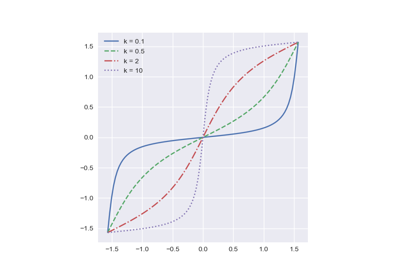
Here’s a plot of our function for varying values of k.

Plot of atan( k tan(x) ) for varying k

Each is fairly flat in the middle, with slope equal to its value of k.

As k increases, f(x; k) becomes more and more like a step function, equal to -π/2 for negative x and π/2 for positive x, i.e.

arctan( k tan(x) ) ≈ sgn(x) π/2

for large k. Here again we might have discussion like above.

Novice: Set k = ±∞. Then ±∞ tan(x) = ±∞ and arctan(±∞) = ±π/2.
Journeyman: You can’t do that!
Expert: Well, you can if you interpret everything in terms of limits.

Orbital resonance in Neptune’s moons

Posted on 17 November 2019 by John

Phys.com published an article a couple days ago NASA finds Neptune moons locked in ‘dance of avoidance’. The article is based on the scholarly paper Orbits and resonances of the regular moons of Neptune.

The two moons closest to Neptune, named Naiad and Thalassa, orbit at nearly the same distance, 48,224 km for Naiad and 50,074 km for Thalassa. However, the moons don’t come as close to each other as you would expect from looking just at the radii of their orbits.

Although the radii of the orbits differ by 1850 km, the two moons do not get closer than about 2800 km apart. The reason has to do with the inclination of the two orbital planes with each other, and a resonance between their orbital periods. When the moons approach each other, one dips below the other, increasing their separation.

Assume the orbits of both moons are circular. (They very nearly are, with major and minor axes differing by less than a kilometer.) Also, choose a coordinate system so that Thalassa orbits in the xy plane. The position of Thalassa at time t is

r_T (cos 2πt/T_T, sin 2πt/T_T, 0)

where r_T is the radius of Thalassa’s orbit and T_T is its period.

The orbit of Naiad is inclined to that of Thalassa by an angle u. The position of Naiad at time t is

r_N (cos u cos 2πt/T_N, sin 2πt/T_N, -sin u cos 2πt/T_N).

I tried implementing the model above using data from Wikipedia articles on the two moons, but in my calculations the moons get closer than reported. I suspect the parameters have to be set carefully in order to demonstrate the kind of resonance we see in observation, and we don’t know these parameters accurately enough to make a direct geometric approach like this work.

from numpy import *

# Orbital radii in km 
r_T = 50074.44
r_N = 48224.41

# Period in days
T_T = 0.31148444
T_N = 0.29439580

def thalassa(t):

    # frequency
    f = 2*pi/T_T

    return r_T * array([
        cos(f*t),
        sin(f*t),
        0
    ])

def naiad(t):
    
    # inclination in radians relative to Thalassa
    i = 0.082205
    
    # frequency
    f = 2*pi/T_N

    return r_N * array([
        cos(i)*cos(f*t),
        sin(f*t),
        -sin(i)*cos(f*t)
    ])

def dist(t):
    return sum((naiad(t) - thalassa(t))**2)**0.5

d = [dist(t) for t in linspace(0, 10*73*T_N, 1000)]
print(d[0], min(d))

In this simulation, the moons are 4442 km apart when t = 0, but this is not the minimum distance. The code above shows an instance where the distance is 2021 km. I tried minor tweaks, such as adding a phase shift to one of the planets or varying the angle of inclination, but I didn’t stumble on anything that cane closer to reproducing the observational results. Maybe resonance depends on factors I’ve left out. Naiad and Thalassa are practically massless compared to Neptune, but perhaps the simulation needs to account for their mass.

The periods of the two moons are nearly in a ratio of 69 to 73. We could idealize the problem by making the periods rational numbers in exactly a ratio of 69 to 73. Then the system would be exactly periodic, and we could find the minimum distance. Studying a model system close to the real one might be useful. If we do tweak the periods, we’d need to tweak the radii as well so that Kepler’s third law applies, i.e. we’d need to keep the squares of the periods proportional to the cubes of the radii.

Related post: Average distance between planets

The hardest logarithm to compute

Posted on 16 November 2019 by John

Suppose you want to compute the natural logarithms of every floating point number, correctly truncated to a floating point result. Here by floating point number we mean an IEEE standard 64-bit float, what C calls a double. Which logarithm is hardest to compute?

We’ll get to the hardest logarithm shortly, but we’ll first start with a warm up problem. Suppose you needed to compute the first digit of a number z. You know that z equals 2 + ε where ε is either 10⁻¹⁰⁰ or −10⁻¹⁰⁰. If ε is positive, you should return 2. If ε is negative, you should return 1. You know z to very high precision a priori, but to return the first digit correctly, you need to compute z to 100 decimal places.

In this post we’re truncating floating point numbers, i.e. rounding down, but similar considerations apply when rounding to nearest. For example, if you wanted to compute 0.5 + ε rounded to the nearest integer.

In general, it may not be possible to know how accurately you need to compute a value in order to round it correctly. William Kahan called this the table maker’s dilemma.

Worst case for logarithm

Lefèvre and Muller [1] found that the floating point number whose logarithm is hardest to compute is

x = 1.0110001010101000100001100001001101100010100110110110 × 2⁶⁷⁸

where the fractional part is written in binary. The log of x, again written in binary, is

111010110.0100011110011110101110100111110010010111000100000000000000000000000000000000000000000000000000000000000000000111 …

The first 53 significant bits, all the bits a floating point number can represent [2], are followed by 65 zeros. We have to compute the log with a precision of more than 118 bits in order to know whether the last bit of the fraction part of the float representation should be a 0 or a 1. Usually you don’t need nearly that much precision, but this is the worst case.

Mathematica code

Here is Mathematica code to verify the result above. I don’t know how to give Mathematica floating point numbers in binary, but I know how to give it integers, so I’ll multiply the fraction part by 2⁵² and take 52 from the exponent.

n = FromDigits[
  "10110001010101000100001100001001101100010100110110110", 2]
x = n  2^(678 - 52)
BaseForm[N[Log[x], 40], 2]

This computes the log of x to 40 significant decimal figures, between 132 and 133 bits, and gives the result above.

A few days ago I wrote about another example by Jean-Michel Muller: A floating point oddity.

William Kahan also came up recently in my post on summing an array of floating point numbers.

***

[1] Vincent Lefèvre, Jean-Michel Muller. Worst Cases for Correct Rounding of the Elementary Functions in Double Precision. November 2000. Research Report 2000-35. Available here.

[2] There are 52 bits in the faction of an IEEE double. The first bit of a fraction is 1, unless a number is subnormal, so the first bit is left implicit, squeezing out one extra bit of precision. That is, storing 52 bits gives us 53 bits of precision.

Hand-drawn Graphviz diagrams

Posted on 13 November 2019 by John

The Sketchviz site lets you enter GraphViz code and get out something that looks hand-drawn. I decided to try it on some of the GraphViz diagrams I’ve made for this blog.

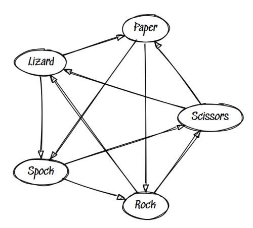
Here’s a diagram from my post on Rock, Paper, Scissors, Lizard, Spock.

The Sketchviz site defaults to Tinos font, which does not look hand-drawn. Maybe you’d want that sometimes: neatly typeset labels and hand-drawn boxes and arrows. In my case, I thought it looked better to use Sedgwick Ave which looks closer to handwriting.

***

Some posts with GraphViz diagrams:

Some of these posts include GraphViz source.

Permutation distance

Posted on 13 November 2019 by John

If you have two sequences, and one is a permutation of the other, how do you measure how far apart the two sequences are?

This post was motivated by the previous post on anagram statistics. For a certain dictionary, the code used in that post found that the longest anagram pairs were the following:

certifications, rectifications
impressiveness, permissiveness
teaspoonsful, teaspoonfuls

Anagrams are more amusing when the two words are more dissimilar, at least in my opinion.

There are several ways to measure (dis)similarity. The words in the first two pairs above are dissimilar in meaning, but the words in the last pair are synonyms [1]. The pairs of words above are not that dissimilar as character strings.

It would be hard to quantify how dissimilar two words are in meaning, but easier to quantify how dissimilar they are as sequences of characters. We’ll look at two approaches: Hamming distance and transposition distance.

Hamming distance

The Hamming distance between two words is the number of positions in which they differ. We can see the Hamming distances between the words above by viewing them in a fixed-width font.

certifications
rectifications

impressiveness
permissiveness

teaspoonsful
teaspoonfuls

The Hamming distances above are 2, 5, and 4.

The anagrams with maximum Hamming distance in my dictionary are “imperfections” and “perfectionism.” (There’s something poetic about these words being anagrams.) The Hamming distance is 13 because these 13-letter words differ in every position.

imperfections
perfectionism

Transposition distance

Another way to measure the distance between two permutations is how many elements would have to be swapped to turn one list into the other. This is called the transposition distance. For example, the transposition distance between “certifications” and “rectifications” is 1, because you only need to swap the first and third characters to turn one into the other.

It’s not so obvious what the transposition distance is between “impressiveness” and “permissiveness”. We can find an upper bound on the distance by experimentation. The two words only differ in the first five letters, so the distance between “impressiveness” and “permissiveness” is no larger than the distance between “impre” and “permi”. The latter pair of words are no more than 4 transpositions apart as the following sequence shows:

impre
pmire
peirm
perim
permi

But is there a shorter sequence of transpositions? Would it help if we used the rest of the letters “ssiveness” as working space?

Computing transposition distance is hard, as in NP-hard. This is unfortunate since transposition has more practical applications than just word games. It is used, for example, in genetic research. It may be practical to compute for short sequences, but in general one must rely on bounds and approximations.

Note that transposition distance allows swapping any two elements. If we only allowed swapping consecutive elements, the problem is much easier, but the results are not the same. When restricted to consecutive swaps, the distance between “certifications” and “rectifications” is 3 rather than 1. We can swap the “c” and the “r” to turn “cer” into “rec” so we have to do something like

cer
ecr
erc
rec

I don’t know a name for the distance where you allow rotations. The words “teaspoonsful” and “teaspoonfuls” differ by one rotation, turning “sful” into “fuls.” While this can be done in one rotation, it would take several swaps.

[1] Although “teaspoonfuls” is far more common, I remember a schoolmarm teaching us that this is incorrect.

And I still recoil at “brother in laws” and say “brothers in law” instead; the majority is on my side on this one.

Anagram frequency

Posted on 13 November 2019 by John

An anagram of a word is another word formed by rearranging its letters. For example, “restful” and “fluster” are anagrams.

How common are anagrams? What is the largest set of words that are anagrams of each other? What are the longest words which have anagrams?

You’ll get different answers to these questions depending on what dictionary you use. I started with the american-english dictionary from the Linux package wamerican. This list contains 102,305 words. I removed all words containing an apostrophe so that possessive forms didn’t count as separate words. I then converted all words to lower case and removed duplicates. This reduced the list to 72,276 words.

Next I alphabetized the letters in each word to create a signature. Signatures that appear more than once correspond to anagrams.

Here are the statistics on anagram classes.

    |------+-------|
    | size | count |
    |------+-------|
    |    1 | 62093 |
    |    2 |  3600 |
    |    3 |   646 |
    |    4 |   160 |
    |    5 |    61 |
    |    6 |    13 |
    |    7 |     2 |
    |    8 |     1 |
    |------+-------|

This means that 62,093 words or about 86% are in an anagram class by themselves. So about 14% of words are an anagram of at least one other word.

The largest anagram class had eight members:

least
slate
stael
stale
steal
tales
teals
tesla

Stael is a proper name. Tesla is a proper name, but it is also a unit of magnetic induction. In my opinion, tesla should count as an English word and Stael should not.

My search found two anagram classes of size seven:

pares
parse
pears
rapes
reaps
spare
spear

and

carets
caster
caters
crates
reacts
recast
traces

The longest words in this dictionary that form anagrams are the following, two pair of 14-letter words and one pair of 12-letter words.

certifications, rectifications
impressiveness, permissiveness
teaspoonsful, teaspoonfuls

Dictionary of anagrams

I made a dictionary of anagrams here. Every word which has a anagram is listed, followed by its anagrams. Here are the first few lines:

abby: baby
abeam: ameba
abed: bade, bead
abel: able, bale, bela, elba
abet: bate, beat, beta
abets: baste, bates, beast, beats, betas
abetter: beretta
abhorred: harbored

There is some redundancy in this dictionary for convenience: every word in the list of anagrams will also appear as the first entry on a line.

Here’s the Python code that produced the dictionary.

from collections import defaultdict

lines = open("american-english", "r").readlines()

words = set()
for line in lines:
    if "'" not in line:
        line = line.strip().lower()
        words.add(line)

def sig(word):
    return "".join(sorted(word))

d = defaultdict(set)
for w in words:
    d[sig(w)].add(w)

for w in sorted(words):
    anas = sorted(d[sig(w)])
    if len(anas) > 1:
        anas.remove(w)
        print("{}: {}".format(w, ", ".join(anas)))

Words with the most consecutive vowels.

A note to new readers

Posted on 12 November 2019 by John

Many of you have been following my blog for years. Thank you for your time and your feedback. But there are always newcomers, and so periodically I like to write a sort of orientation post.

You can subscribe to this blog by RSS or email. I also have a monthly newsletter where I highlight the most popular posts of the month, and occasionally say a little bit about what my business is up to. You can find links to the RSS feed, email subscription, and newsletter here.

I have a lot of specialized Twitter accounts. Most of the content is scheduled, but I sprinkle in spontaneous content occasionally. The accounts are a little broader than their names imply. For example, AlgebraFact mostly posts on algebra and number theory, but it’s also where I post miscellaneous math content. TeXtip posts about LaTeX, but also about typography and Unicode. CompSciFact posts about computer science, and anything else that I think people interested in computer science might want to read.

Sometimes people ask whether I have a team of writers, or they simply assume that I do. Although I work with several other consultants, I write all the blog content and nearly all of Twitter content; I have sent a few tweets that other people have offered for me to use, maybe 20 tweets if I had to guess.

There’s a lot of content on this site that isn’t blog posts. You can find this content via the menu at the top. For example, the technical notes page links to a lot of notes on miscellaneous math and programming topics.

Thanks for reading.

Just evaluating a polynomial: how hard could it be?

Posted on 12 November 2019 by John

The previous post looked at an example of strange floating point behavior taking from book End of Error. This post looks at another example.

This example, by Siegfried Rump, asks us to evaluate

333.75 y⁶ + x² (11 x² y² − y⁶ − 121 y⁴ − 2) + 5.5 y⁸ + x/(2y)

at x = 77617 and y = 33096.

Here we evaluate Rump’s example in single, double, and quadruple precision.

#include <iostream>
#include <quadmath.h>

using namespace std;

template <typename T> T f(T x, T y) {
    T x2 = x*x;
    T y2 = y*y;
    T y4 = y2*y2;
    T y6 = y2*y4;
    T y8 = y2*y6;
    return 333.75*y6 + x2*(11*x2*y2 - y6 - 121*y4 - 2) + 5.5*y8 + x/(2*y);
}

int main() {  

    int x = 77617;
    int y = 33096;
    
    cout << f<float>(x, y) << endl;
    cout << f<double>(x, y) << endl;
    cout << (double) f<__float128>(x, y) << endl;

}

This gives three answers,

-1.85901e+030
-1.18059e+021
1.1726

none of which is remotely accurate. The exact answer is −54767/66192 = −0.827…

Python gives the same result as C++ with double precision, which isn’t surprising since Python floating point numbers are C doubles under the hood.

Where does the problem come from? The usual suspect: subtracting nearly equal numbers. Let’s split Rump’s expression into two parts.

s = 333.75 y⁶ + x²(11x²y² − y⁶ − 121y⁴ − 2)

t = 5.5y⁸ + x/(2y)

and look at them separately. We get

s = -7917111340668961361101134701524942850.00         
t =  7917111340668961361101134701524942849.1726...

The values −s and t agree to 36 figures, but quadruple precision has only 34 figures [1]. Subtracting these two numbers results in catastrophic loss of precision.

Rump went to some effort to conceal what’s going on, and the example is contrived to require just a little more than quad precision. However, his example illustrates things that come up in practice. For one, the values of x and y are not that big, and so we could be mislead into thinking the terms in the polynomial are not that big. For another, it’s not clear that you’re subtracting nearly equal numbers. I’ve been caught off guard by both of these in real applications.

Floating point numbers are a leaky abstraction. They can trip you up if you don’t know what you’re doing. But the same can be said of everything in computing. We can often ignore finite precision just as we can often ignore finite memory, for example. The proper attitude toward floating point numbers is somewhere between blissful ignorance and unnecessary fear.

Floating point oddity

Posted on 11 November 2019 by John

Here is an example fiendishly designed to point out what could go wrong with floating point arithmetic, even with high precision.

I found the following example by Jean-Michel Muller in John Gustafson’s book End of Error. The task is to evaluate the following function at 15, 16, 17, and 9999.

$\begin{align*} e(x) &= \frac{\exp(x) - 1}{x} \\ q(x) &= \left| x - \sqrt{x^2 + 1}\right| - \frac{1}{x + \sqrt{x^2 + 1}} \\ h(x) &= e(q(x)^2) \\ \end{align*}$

Here e(0) is defined by continuity to be 1. That is, we define e(0) to be the limit of e(x) as x approaches 0. That limit exists, and it equals 1, so we define e(0) to be 1.

If you directly implement the functions above in C++, you will get 0 as the output, whether you use single, double, or even quadruple precision as the following code shows. However, the correct answer in each case is 1.

#include <iostream>
#include <math.h>
#include <quadmath.h>

using namespace std;

template <typename T> T e(T x) {
  // See footnote [1]
  return x == 0. ? 1. : (exp(x) - 1.)/x;
}

template <typename T> T q(T x) {
  return fabs(x - sqrt(x*x + 1.)) - 1./(x + sqrt(x*x + 1.));
}

template <typename T> T h(T x) {
  return e( q(x)*q(x) );
}

int main() {

  int x[] = {15, 16, 17, 9999};

  for (int i = 0; i < 4; i++) {
      cout << h(     float(x[i]) ) << endl;
      cout << h(    double(x[i]) ) << endl;
      cout << h(__float128(x[i]) ) << endl;
  }
}

A little algebra [2] shows that the function q(x) would return 0 in exact arithmetic, but not in floating point arithmetic. It returns an extremely small but non-zero number, and the numerator of (exp(x) - 1.)/x evaluates to 0.

If q(x) returned exactly zero, h(x) would correctly return 1. Interestingly, if q(x) were a little less accurate, returning a little larger value when it should return 0, h would be more accurate, returning a value close to 1.

I tried replacing exp(x) - 1 with expm1(x). This made no difference. (More on expm1 here.)

Incidentally, bc -l gives the right result, no matter how small you set scale.

define ee(x) { if (x == 0) return 1 else return (e(x) - 1)/x }
define abs(x) { if (x > 0) return x else return -x }
define q(x) { return abs(x - sqrt(x^2 + 1)) - 1/(x + sqrt(x^2 + 1)) }
define h(x) { return ee( q(x)^2 ) }

Update: See the next post for another example, this time evaluating a polynomial.

[1] Some have suggested that this is a mistake, that you should never test floating point numbers for equality. It’s true that in general you should only test floating point numbers for approximate equality. But the code here is not a mistake; it’s part of the illustration.

[2] Several people have pointed out that you could fix this problem by doing a little algebra. But the point is not to fix it; Muller created this example to show that it is broken. He deliberately obfuscated the problem a little to make a point. This is an artificial example, meant to show in a simple setting the kind of the that could happen in a real problem. Sometimes you may subtract equal or nearly equal things without realizing it.

Mathematical killer apps

Posted on 11 November 2019 by John

A killer app is an program so useful that people will buy a larger system just to use it. For example, the VisiCalc spreadsheet was a killer app for the Apple II, maybe the first program to be called a “killer app.” People would buy an Apple II just so they could run VisiCalc. Microsoft Office is a killer app for Windows: many people run Windows so they can run MS Office.

Calculus

I was thinking about the mathematical analog of killer apps. For example, finding maxima is a killer app for calculus. If that’s all you could do with calculus, we’d still teach calculus. After one semester of calculus, students can easily solve optimization problems that would be virtually impossible otherwise.

Differential equations

Mechanical vibrations are a killer app for differential equations. (Non-mechanical systems such as LRC circuits follow the same equations.) If an engineer applies anything from a differential equation class, this is probably it.

Complex variables

Contour integration is a killer app for complex analysis. There are other applications of complex analysis, but contour integration is certainly one of the big ones.

Lack of killer apps

Some areas of math don’t have a killer app that I can think of. They may have practical application, but there isn’t a particular application that stands out, not one that many people would agree on [1]. If you did a Family Feud-style poll on applications of calculus, differential equations, and complex analysis, I image the examples above would be on the board if not the top result.

Category theory can be useful, but its applications are scattered. If category theory has a killer application, I doubt there’s a consensus of what that application would be.

A killer application is different from a key theorem. I imagine a lot of people would say that the Yoneda lemma is the most important theorem in an introductory course in category theory, but I wouldn’t call it a killer app. My idea of a killer app is something that fills in the blank “You should take a course in X if for no other reason than that you’ll be able to ______.” For instance, many people take a course in statistics just so they can do linear regression.

Discussion

If you have ideas about what killer apps would be in various areas of math, please share them in the comments below.

[1] I’m reminded of someone’s description of G. K. Chesterton as a master who left no masterpiece. That is, he wrote a lot of great lines, but no great book.

Month: November 2019

arctan( k tan(x) )

Related posts

Orbital resonance in Neptune’s moons

The hardest logarithm to compute

Worst case for logarithm

Mathematica code

Related posts

Hand-drawn Graphviz diagrams

Permutation distance

Hamming distance

Transposition distance

Related posts

Anagram frequency

Dictionary of anagrams

Related post

A note to new readers

Just evaluating a polynomial: how hard could it be?

Similar posts

Floating point oddity

Related posts

Mathematical killer apps

Calculus

Differential equations

Complex variables

Lack of killer apps

Discussion

Related posts