Generating all primitive Pythagorean triples with linear algebra

A Pythagorean triple is a set of positive integers that can be the lengths of sides of a right triangle, i.e. numbers a, b, and c such that

a² + b² = c².

A primitive Pythagorean triple (PPT) is a Pythagorean triple whose elements are relatively prime. For example, (50, 120, 130) is a Pythagorean triple, but it’s not primitive because all the entries are divisible by 10. But (5, 12, 13) is a primitive Pythagorean triple.

A method of generating all PPTs has been known since the time of Euclid, but I recently ran across a different approach to generating all PPTs [1].

Let’s standardize things a little by assuming our triples have the form (a, b, c) where a is odd, b is even, and c is the hypotenuse [2]. In every PPT one of the sides is even and one is odd, so we will assume the odd side is listed first.

It turns out that all PPTs can be found by multiplying the column vector [3, 4, 5] repeatedly by matrices M0, M1, or M2. In [1], Romik uses the sequence of matrix multiplications needed to create a PPT as trinary number associated with the PPT.

The three matrices are given as follows.

\begin{align*} M_0 &= \begin{bmatrix} \phantom{-}1 & \phantom{-}2 & \phantom{-}2 \\ \phantom{-}2 & \phantom{-}1 & \phantom{-}2 \\ \phantom{-}2 & \phantom{-}2 & \phantom{-}3 \end{bmatrix} \\ M_1 &= \begin{bmatrix} -1 & \phantom{-}2 & \phantom{-}2 \\ -2 & \phantom{-}1 & \phantom{-}2 \\ -2 & \phantom{-}2 & \phantom{-}3 \end{bmatrix} \\ M_2 &= \begin{bmatrix} \phantom{-}1 & -2 & \phantom{-}2 \\ \phantom{-}2 & -1 & \phantom{-}2 \\ \phantom{-}2 & -2 & \phantom{-}3 \end{bmatrix} \end{align*}

Note that all three matrices have the same entries, though with different signs. If you number the columns starting at 1 (as mathematicians commonly do and computer scientists may not) then Mk is the matrix whose kth column is negative. There is no 0th column, so M0 is the matrix with no negative columns. The numbering I’ve used here differs from that used in [1].

For example, the primitive Pythagorean triple [5, 12, 13] is formed by multiplying [3, 4, 5] on the left by M2. The PPT [117, 44, 125] is formed by multiplying [3, 4, 5] by
M1 M1 M2.

\begin{bmatrix} 117 \\ 44 \\ 125 \end{bmatrix} = M_1 M_1 M_2 \begin{bmatrix} 3 \\ 4 \\ 5 \end{bmatrix}

More Pythagorean posts

[1] The dynamics of Pythagorean triples by Dan Romik

[2] Either a is odd and b is even or vice versa, so we let a be the odd one.

If a and b were both even, c would be even, and the triple would not be primitive. If a and b were both odd, c² would be divisible by 2 but not by 4, and so it couldn’t be a square.

Playing around with a rational rose

A “rose” in mathematics is typically a curve with polar equation

r = cos(kθ)

where k is a positive integer. If k is odd, the resulting graph has k “petals” and if k is even, the plot has 2k petals.

Sometimes the term rose is generalized to the case of non-integer k. This is the sense in which I’m using the phrase “rational rose.” I’m not referring to an awful piece of software by that name [1]. This post will look at a particular rose with k = 2/3.

My previous post looked at

r = cos(2θ/3)

and gave the plot below.

Plot of r = abs(cos(2 theta / 2) )

Unlike the case where k is an integer, the petals overlap.

In this post I’d like to look at two things:

  1. The curvature in the figure above, and
  2. Differences between polar plots in Python and Mathematica

Curvature

The graph above has radius 1 since cosine ranges from −1 to 1. The curve is made of arcs that are approximately circular, with the radius of these approximating circles being roughly 1/2, sometimes bigger and sometimes smaller. So we would expect the curvature to oscillate roughly around 2. (The curvature of a circle of radius r is 1/r.)

The curvature can be computed in Mathematica as follows.

    numerator = D[x[t], {t, 1}] D[y[t], {t, 2}] - 
                D[x[t], {t, 2}] D[y[t], {t, 1}]
    denominator = (D[x[t], t]^2 + D[y[t], t]^2)^(3/2)
    Simplify[numerator / denominator]

This produces

\kappa = \frac{3 \sqrt{2} \left(5 \cos \left(\dfrac{4 \theta}{3}\right)+21\right)}{\left(5 \cos \left(\dfrac{4 \theta}{3}\right)+13\right)^{3/2}}

A plot shows that the curvature does indeed oscillate roughly around 2.

The minimum curvature is 13/9, which the curve takes on at polar coordinate (1, 0), as well as at other points. That means that the curve starts out like a circle of radius 9/13 ≈ 0.7.

The maximum curvature is 3 and occurs at the origin. There the curve is approximately a circle of radius 1/3.

Matplotlib vs Mathematica

To make the plot we’ve been focusing on, I plotted

r = cos(2θ/3)

in Mathematica, but in matplotlib I had to plot

r = |cos(2θ/3)|.

In both cases, θ runs from 0 to 8π. To highlight the differences in the way the two applications make polar plots, let’s plot over 0 to 2π with both.

Mathematica produces what you might expect.

    PolarPlot[Cos[2 t/3], {t, 0, 2 Pi}]

Mathematica plot of Cos[2 theta/3]

Matplotlib produces something very different. It handles negative r values by moving the point r = 0 to a circle in the middle of the plot. Notice the r-axis labels at about 22° running from −1 to 1.

    theta = linspace(0, 2*pi, 1000)
    plt.polar(theta, cos(2*theta/3))

Python plot of cos( 2 theta / 3 )

Note also that in Mathematica, the first argument to PolarPlot is r(θ) and the second is the limits on θ. In matplotlib, the first argument is θ and the second argument is r(θ).

Note that in this particular example, taking the absolute value of the function being plotted was enough to make matplotlib act like I expected. That’s only happened true when plotted over the entire range 0 to 8π. In general you have to do more work than this. If we insert absolute value in the plot above, still plotting from 0 to 2π, we do not reproduce the Mathematca plot.

    plt.polar(theta, abs(cos(2*theta/3)))

More polar coordinate posts

[1] Rational Rose was horribly buggy when I used it in the 1990s. Maybe it’s not so buggy now. But I imagine I still wouldn’t like the UML-laden style of software development it was built around.

Quatrefoils

I was reading The 99% Invisible City this evening, and there was a section on quatrefoils. Here’s an example of a quatrefoil from Wikipedia.

quatrefoil

There’s no single shape known as a quatrefoil. It’s a family of shapes that look something like the figure above.

I wondered how you might write a fairly simple mathematical equation to draw a quatrefoil. Some quatrefoils are just squares with semicircles glued on their edges. That’s no fun.

Here’s a polar equation I came up with that looks like a quatrefoil, if you ignore the interior lines.

This is the plot of r = cos(2θ/3).

Plot of r = abs(cos(2 theta / 2) )

Update: Based on a suggestion in the comments, I’ve written another post on quatrefoils using an equation that has a parameter to control the shape.

Kronecker sum

I’m working on a project these days that uses four different kinds of matrix product, which made me wonder if there’s another kind of product out there that I could find some use for.

In the process of looking around for other matrix products, I ran across the Kronecker sum. I’ve seen Kronecker products many times, but I’d never heard of Kronecker sums.

The Kronecker sum is defined in terms of the Kronecker product, so if you’re not familiar with the latter, you can find a definition and examples here. Essentially, you multiply each scalar element of the first matrix by the second matrix as a block matrix.

The Kronecker product of an m × n matrix A and a p × q matrix B is a mp × nq matrix KA B. You could think of K as an m × n matrix whose entries are p × q blocks.

So, what is the Kronecker sum? It is defined for two square matrices, an n × n matrix A and an m × m matrix B. The sizes of the two matrices need not match, but the matrices do need to be square.  The Kronecker sum of A and B is

AB = AIm + InB

where Im and In are identity matrices of size m and n respectively.

Does this make sense dimensionally? The left side of the (ordinary) matrix addition is nm × nm, and so is the right side, so the addition makes sense.

However, the Kronecker sum is not commutative, and usually things called “sums” are commutative. Products are not always commutative, but it goes against convention to call a non-commutative operation a sum. Still, the Kronecker sum is kinda like a sum, so it’s not a bad name.

I don’t have any application in mind (yet) for the Kronecker sum, but presumably it was defined for a good reason, and maybe I’ll run an application, maybe even on the project alluded to at the beginning.

There are several identities involving Kronecker sums, and here’s one I found interesting:

exp( A ) ⊗ exp( B ) = exp( A B ).

If you haven’t seen the exponential of a matrix before, basically you stick your matrix into the power series for the exponential function.

Examples

First, let’s define a couple matrices A and B.

\begin{align*} A &= \left( \begin{array}{cc} 1 & 2 \\ 3 & 4 \\ \end{array} \right) \\ B &= \left( \begin{array}{ccc} 1 & 0 & 1 \\ 1 & 2 & 0 \\ 2 & 0 & 3 \\ \end{array} \right) \end{align*}

We can compute the Kronecker sums

S = AB

and

T = B ⊕ A

with Mathematica to show they are different.

    A = {{1, 2}, {3, 4}}
    B = {{1, 0, 1}, {1, 2, 0}, {2, 0, 3}}
    S = KroneckerProduct[A, IdentityMatrix[3]] + 
        KroneckerProduct[IdentityMatrix[2], B]
    T = KroneckerProduct[B, IdentityMatrix[2]] + 
        KroneckerProduct[IdentityMatrix[3], A]

This shows

\begin{align*} A \oplus B &= \left( \begin{array}{cccccc} 2 & 0 & 1 & 2 & 0 & 0 \\ 1 & 3 & 0 & 0 & 2 & 0 \\ 2 & 0 & 4 & 0 & 0 & 2 \\ 3 & 0 & 0 & 5 & 0 & 1 \\ 0 & 3 & 0 & 1 & 6 & 0 \\ 0 & 0 & 3 & 2 & 0 & 7 \\ \end{array} \right) \\ B \oplus A &= \left( \begin{array}{cccccc} 2 & 2 & 0 & 0 & 1 & 0 \\ 3 & 5 & 0 & 0 & 0 & 1 \\ 1 & 0 & 3 & 2 & 0 & 0 \\ 0 & 1 & 3 & 6 & 0 & 0 \\ 2 & 0 & 0 & 0 & 4 & 2 \\ 0 & 2 & 0 & 0 & 3 & 7 \\ \end{array} \right) \end{align*}

and so the two matrices are not equal.

We can compute the matrix exponentials of A and B with the Mathematica function MatrixExp to see that

\begin{align*} \exp(A) &= \left( \begin{array}{cc} 2.71828 & 7.38906 \\ 20.0855 & 54.5982 \\ \end{array} \right) \\ \exp(B) &= \left( \begin{array}{ccc} 2.71828 & 1. & 2.71828 \\ 2.71828 & 7.38906 & 1. \\ 7.38906 & 1. & 20.0855 \\ \end{array} \right) \end{align*}

(I actually used MatrixExp[N[A]] and similarly for B so Mathematica would compute the exponentials numerically rather than symbolically. The latter takes forever and it’s hard to read the result.)

Now we have

\begin{align*} \exp(A) \otimes \exp(B) &= \left( \begin{array}{cccccc} 512.255 & 0. & 606.948 & 736.673 & 0. & 872.852 \\ 361.881 & 384.002 & 245.067 & 520.421 & 552.233 & 352.431 \\ 1213.9 & 0. & 1726.15 & 1745.7 & 0. & 2482.38 \\ 1105.01 & 0. & 1309.28 & 1617.26 & 0. & 1916.22 \\ 780.631 & 828.349 & 528.646 & 1142.51 & 1212.35 & 773.713 \\ 2618.55 & 0. & 3723.56 & 3832.45 & 0. & 5449.71 \\ \end{array} \right) \\ \exp(A \oplus B) &= \left( \begin{array}{cccccc} 512.255 & 0. & 606.948 & 736.673 & 0. & 872.852 \\ 361.881 & 384.002 & 245.067 & 520.421 & 552.233 & 352.431 \\ 1213.9 & 0. & 1726.15 & 1745.7 & 0. & 2482.38 \\ 1105.01 & 0. & 1309.28 & 1617.26 & 0. & 1916.22 \\ 780.631 & 828.349 & 528.646 & 1142.51 & 1212.35 & 773.713 \\ 2618.55 & 0. & 3723.56 & 3832.45 & 0. & 5449.71 \\ \end{array} \right) \end{align*}

and so the two matrices are equal.

Even though the identity

exp( A ) ⊗ exp( B ) = exp( A B )

may look symmetrical, it’s not. The matrices on the left do not commute in general. And not only are AB and BA different in general, their exponentials are also different. For example

\exp(B\oplus A) = \left( \begin{array}{cccccc} 512.255 & 736.673 & 0. & 0. & 606.948 & 872.852 \\ 1105.01 & 1617.26 & 0. & 0. & 1309.28 & 1916.22 \\ 361.881 & 520.421 & 384.002 & 552.233 & 245.067 & 352.431 \\ 780.631 & 1142.51 & 828.349 & 1212.35 & 528.646 & 773.713 \\ 1213.9 & 1745.7 & 0. & 0. & 1726.15 & 2482.38 \\ 2618.55 & 3832.45 & 0. & 0. & 3723.56 & 5449.71 \\ \end{array} \right)

Related posts

Nonlinear mod 5

This post is a follow-on to the previous post on perfectly nonlinear functions. In that post we defined a way to measure the degree of nonlinearity of a function between two Abelian groups. We looked at functions that take sequences of four bits to a single bit. In formal terms, our groups were GF(24) and GF(2).

In this post we’ll start out by looking at integers mod 5 to show how the content of the previous post takes a different form in different groups. Sometimes the simplicity of working in binary makes things harder to see. For example, we noted in the previous post that the distinction between addition and subtraction didn’t matter. It matters in general!

Let B be the group of integers mod 5 and A the group of pairs of integers mod 5. That is, A is the direct product B × B. We will compute the uniformity of several functions from A to B. (Recall that less uniformity means more nonlinearity.) Then we’ll conclude by looking what happens if we work modulo other integers.

Python code

Here’s the code we’ll use to compute uniformity.

    from itertools import product
    from numpy import array

    m = 5
    r = range(m)

    def deriv(f, x, a):
        return (f(x + a) - f(x))%m

    def delta(f, a, b):
        return {x for x in product(r, r) if all(deriv(f, array(x), a) == b)}

    def uniformity(f):
        u = 0
        for a in product(r, r):
            if a == (0, 0):
                continue
            for b in product(r, r):
                t = len(delta(f, array(a), array(b)))
                if t > u:
                    u = t
        return u

We didn’t call attention to it last time, but the function f(x + a) – f(x) is called a derivative of f, and that’s why we named the function above deriv.

Here are a few functions whose uniformity we’d like to compute.

    # (u, v) -> u^2 + v^2 
    def F2(x): return sum(x**2)%m

    # (u, b) -> u^3 + v^3 
    def F3(x): return sum(x**3)%m

    # (u, b) -> u^2 + v
    def G(x):  return (x[0]**2 + x[1])%m

    # (u, v) -> uv
    def H(x):  return (x[0]*x[1])%m

Now let’s look at their uniformity values.

    print( uniformity(F2) )
    print( uniformity(F3) )
    print( uniformity(G) )
    print( uniformity(H) )

Results mod 5

This prints out 5, 10, 25, and 5. This says that the functions F2 and H are the most nonlinear, in fact “perfectly nonlinear.” The function G, although nonlinear, has the same uniformity as a linear function.

The function F3 may be the most interesting, having intermediate uniformity. In some sense the sum of cubes is closer to being a linear function than the sum of squares is.

Other moduli

We can easily look at other groups by simply changing the value of m at the top of the code.

If we set the modulus to 7, we get analogous results. The uniformities of the four functions are 7, 14, 49, and 7. They’re ranked exactly as they were when the modulus was 5.

But that’s not always the case for other moduli as you can see in the table below. Working mod 8, for example, the sum of squares is more uniform than the sum of cubes, the opposite of the case mod 5 or mod 7.

    |----+-----+-----+-----+----|
    |  m |  F2 |  F3 |   G |  H |
    |----+-----+-----+-----+----|
    |  2 |   4 |   4 |   4 |  2 |
    |  3 |   3 |   9 |   9 |  3 |
    |  4 |  16 |   8 |  16 |  8 |
    |  5 |   5 |  10 |  25 |  5 |
    |  6 |  36 |  36 |  36 | 18 |
    |  7 |   7 |  14 |  49 |  7 |
    |  8 |  64 |  32 |  64 | 32 |
    |  9 |  27 |  81 |  81 | 27 |
    | 10 | 100 | 100 | 100 | 50 |
    | 11 |  11 |  22 | 121 | 11 |
    | 12 | 144 | 144 | 144 | 72 |
    |----+-----+-----+-----+----|

In every case, G is the most uniform function and H is the least. Also, G is strictly more uniform than H. But there are many different ways F2 and F3 can fit between G and H.

Perfectly nonlinear functions

The other day I heard someone suggest that a good cocktail party definition of cryptography is puzzle making. Cryptographers create puzzles that are easy to solve given the key, but ideally impossible without the key.

Linearity is very useful in solving puzzles, and so a puzzle maker would like to create functions that are as far from linear as possible. That is why cryptographers are interested in perfectly nonlinear functions (PNs) and almost perfect nonlinear functions (APNs), which we will explore here.

The functions we are most interested in map a set of bits to a set of bits. To formalize things, we will look at maps between two finite Abelian groups A and B. If we look at lists of bits with addition defined as component-wise XOR [1], we have an Abelian group, but the ideas below apply to other kinds of Abelian groups as well.

We will measure the degree of nonlinearity of a function F from A to B by the size of the sets

\delta(a, b) = \{x \mid F(a + x) - F(x) = b\}

where a and x are in A and b is in B [2].

If F is a linear function, F(a + x) = F(a) + F(x), and so δ(a, b) simplifies to

\delta(a, b) = \{x \mid F(a) = b\}

which equals all of the domain A, if F(a) = b. So for linear functions, the set δ(a, b) is potentially as large as possible, i.e. all of A. Perfectly nonlinear functions will be functions where the sets δ(a, b) are as small as possible, and almost perfectly nonlinear functions will be functions were δ(a, b) is as small as possible in a given context.

The uniformity of a function F is defined by

\underset{a \ne 0}{\max_{a \in A, \, b\in B}} \,\, |\delta(a,b)|

The restriction a ≠ 0 is necessary since otherwise the uniformity of every function would be the same.

For linear functions, the uniformity is as large as possible, i.e. |A|. As we will show below, a nonlinear function can have maximum uniformity as well, but some nonlinear functions have smaller uniformity. So some nonlinear functions are more nonlinear than others.

We will compute the uniformity of a couple functions, mapping 4 bits to 1 bit, with the following Python code.

    A = range(16)
    B = range(2)
    nonZeroA = range(1, 16)

    def delta(f, a, b):
        return {x for x in A if f(x^a) ^ f(x) == b}

    def uniformity(f):
        return max(len(delta(f, a, b)) for a in nonZeroA for b in B)

We could look at binary [3] functions with domains and ranges of different sizes by changing the definitions of A, B, and nonZeroA.

Note that in our groups, addition is component-wise XOR, denoted by ^ in the code above, and that subtraction is the same as addition since XOR is its own inverse. Of course in general addition would be defined differently and subtraction would not be the same as addition. When working over a binary field, things are simpler, sometimes confusingly simpler.

We want to compute the uniformity of two functions. Given bits x0, x1, x2, and x3, we define

F(x0, x1, x2, x3) = x0 x1

and

G(x0, x1, x2, x3) = x0 x1 + x2 x3.

We can implement these in Python as follows.

    def F(x):
        x = [c == '1' for c in format(x, "04b")]
        return x[0] and x[1]

    def G(x):
        x = [c == '1' for c in format(x, "04b")]
        return (x[0] and x[1]) ^ (x[2] and x[3])

Next we compute the uniformity of the two functions.

    print( uniformity(F) )
    print( uniformity(G) )

This shows that the uniformity of F is 16 and the uniformity of G is 8. Remember that functions with smaller uniformity are considered more nonlinear. Both functions F and G are nonlinear, but G is more nonlinear in the sense defined here.

To see that F is nonlinear, let x = (1, 0, 0, 0) and y = (0, 1, 0, 0).

1 = F(x + y) ≠ F(x) + F(y) = 0.

It turns out that 8 is the smallest possible uniformity for a function from 4 bits to 1 bit, and the function G is said to be perfectly nonlinear.

I haven’t defined perfect nonlinearity or almost perfect nonlinearaity precisely, only saying that they have something to do with maximum nonlinearity (minimum uniformity) in some context. I may say more about that context in a future post.

Related posts

[1] XOR stands for exclusive or. For Boolean variables p and q, p XOR q is true if either p is true or q is true, but not both. The component-wise XOR of two binary numbers sets each bit of the result to the XOR of the corresponding input bits. For example, 1001 XOR 1010 = 0011.

[2] This definition comes from Perfect nonlinear functions and cryptography by Céline Blondeau and Kaisa Nyberg.

[3] The next post replaces binary numbers with base 5 and other bases.
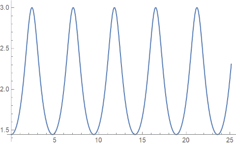
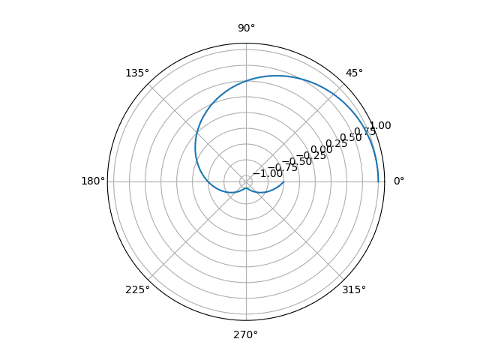
Python one-liner to print Roman numerals

Here’s an amusing little Python program to convert integers to Roman numerals:

    def roman(n): print(chr(0x215F + n))

It only works if n is between 1 and 12. That’s because Unicode contains characters for the Roman numerals I through XII.

Here are the characters it produces:

Ⅰ Ⅱ Ⅲ Ⅳ Ⅴ Ⅵ Ⅶ Ⅷ Ⅸ Ⅹ Ⅺ Ⅻ

You may not be able to see these, depending on what fonts you have installed. I can see them in my browser, but when I ran the code above in a terminal window I only saw a missing glyph placeholder.

If you can be sure your reader can see the characters, say in print rather than on the web, the single-character Roman numerals look nice, and they make it clear that they’re to be interpreted as Roman numerals.

Here’s a screenshot of the symbols.

I II III IV V VI VII VIII IX X XI XII


Bidirectional text

This post will take a look at simple bidirectional text, such as a bit of English inside an Arabic document, or a few words of Hebrew inside a French document. If you want to explore the subject in all its complexity, see Unicode Standard Annex 9.

You may not need to do anything special to display bidirectional text. For example, when I typed the following sentence, I just typed the letters in logical order.

The first letter of the Hebrew alphabet is אלף.

For the last word, I typed א, then ל, then ף. When I entered the ל, the editor put it on the left side of the א, and when I entered ף the editor put it to the left of the ל. The characters are stored in memory in the same sequence that I typed them, though they are displayed in the order appropriate for each language.

You can change the default display ordering of characters by inserting control characters. For example, I typed

The [U+202E]quick brown fox[U+202C] jumped.

and the text displays [1] as

The ‮quick brown fox‬ jumped.

The Unicode character U+202E, known as RLO for “right-to-left override,” tells the browser to display the following letters from right-to-left. Then the character U+202C, known as PDF for “pop directional formatting,” exits that mode, returning to left-to-right [2]. If we copy the first sentence into a text file and open it with a hex editor we can see the control characters, circled in red.

hex editor screen shot

I saved the file in UTF-16 encoding to make the characters easy to see: each quartet of hex characters represented a Unicode character. UTF-8 encoding more common and more compressed.

If for some reason you wanted to force Hebrew to display from left-to-right, you could insert U+202D, known as LRO for “left-to-right override.” The character to exit this mode is PDF, U+202C, as before.

Here’s a bit of Hebrew written left-to-right:

Written left-to-right: ‭אלף.

And here’s what it looks like in an hex editor:

another hex editor screen shot

Related posts

[1] This should look the same as

The xof nworb kciuq jumped.

though in this footnote I typed the letters in the order they appear: xof …

If for some reason the text in the body of the post displays in normal order, not as in this note, then something has gone wrong with your browser’s rendering.

[2] So in addition to Portable Document Format and Probability Density Function, PDF can stand for Pop Directional Formatting. Here “pop” is being used in the computer science sense of popping a stack.

Understanding statistical error

A simple linear regression model has the form

y = μ + βx + ε.

This means that the output variable y is a linear function of the input variable x, plus some error term ε that is randomly distributed.

There’s a common misunderstanding over whose error the error term is. A naive view is that the world really is linear, that

y = μ + βx

is some underlying Platonic reality, and that the only reason that we don’t measure exactly that linear part is that we as observers have made some sort of error, that the fault is the real world rather than in the model.

No, reality is what it is, and it’s our model that is in error. Some aspect of reality may indeed have a structure that is approximately linear (over some range, under some conditions), but when we truncate reality to only that linear approximation, we introduce some error. This error may be tolerable—and thankfully it often is—but the error is ours, not the world’s.

Why a little knowledge is a dangerous thing

Alexander Pope famously said

A little learning is a dangerous thing;
Drink deep, or taste not the Pierian spring:
There shallow draughts intoxicate the brain,
And drinking largely sobers us again.

I’ve been thinking lately about why a little knowledge is often a dangerous thing, and here’s what I’ve come to.

Any complex system has many causes acting on it. Some of these are going to be more legible than others. Here I’m using “legible” in a way similar to how James Scott uses the term. As Venkatesh Rao summarizes it,

A system is legible if it is comprehensible to a calculative-rational observer looking to optimize the system from the point of view of narrow utilitarian concerns and eliminate other phenomenology. It is illegible if it serves many functions and purposes in complex ways, such that no single participant can easily comprehend the whole. The terms were coined by James Scott in Seeing Like a State.

People who have a little knowledge of a subject are only aware of some of the major causes that are acting, and probably they are aware of the most legible causes. They have an unbalanced view because they are aware of the forces pushing in one direction but not aware of other forces pushing in other directions.

A naive view may be unaware of a pair of causes in tension, and may thus have a somewhat balanced perspective. And an expert may be aware of both causes. But someone who knows about one cause but not yet about the other is unbalanced.

Examples

When I first started working at MD Anderson Cancer Center, I read a book on cancer called One Renegade Cell. After reading the first few chapters, I wondered why we’re not all dead. It’s easy to see how cancer can develop from one bad cell division and kill you a few weeks later. It’s not as easy to understand why that doesn’t usually happen. The spreading of cancer is more legible than natural defenses against cancer.

I was recently on the phone with a client who had learned enough about data deidentification to become worried. I explained that there were also reasons to not be as worried, but that they’re more complicated, less legible.

What to do

Theories are naturally biased toward causes that are amenable to theory, toward legible causes. Practical experience and empirical data tend to balance out theory by providing some insight into less legible causes.

A little knowledge is dangerous not so much because it is partial but because it is biased; it’s often partial in a particular way, such as theory lacking experience. If you spiral in on knowledge in a more balanced manner, with a combination of theory and experience, you might not be as dangerous along the way.

When theory and reality differ, the fault lies in the theory. More on that in my next post. Theory necessarily leaves out complications, and that’s what makes it useful. The art is knowing which complications can be safely ignored under which circumstances.

Related posts