Justifying separation of variables

The separation of variables technique for solving partial differential equations looks like a magic trick the first time you see it. The lecturer, or author if you’re more self-taught, makes an audacious assumption, like pulling a rabbit out of a hat, and it works.

For example, you might first see the heat equation

ut = c² uxx.

The professor asks you to assume the solution has the form

u(x, t) = X(x) T(t).

i.e. the solution can be separated into the product of a function of x alone and a function of t alone.

Following that you might see Laplace’s equation on a rectangle

uxx + uyy = 0

with the analogous assumption that

u(x, y) = X(x) Y(y),

i.e. the product of a function of x alone and a function of y alone.

There are several possible responses to this assumption.

  1. Whatever you say, doc.
  2. How can you assume that?
  3. How do you know you’re not missing any possibilities?
  4. What made someone think to try this?

As with many things, separation of variables causes the most consternation for the moderately sophisticated students. The least sophisticated students are untroubled, and the most sophisticated student can supply their own justification (at least after the fact).

One response to question (2) is “Bear with me. I’ll show that this works.”

Another response would be “OK, how about assuming the solution is a sum of such functions. That’s a much larger space to look in. And besides, we are going to take sums of such solutions in a few minutes.” One could argue from functional analysis or approximation theory that the sums of separable functions are dense in reasonable space of functions [1].

This is a solid explanation, but it’s kind of anachronistic: most students see separation of variables long before they see functional analysis or approximation theory. But it would be a satisfying response for someone who is seeing all this for the second time. Maybe they were exposed to separation of variables as an undergraduate and now they’re taking a graduate course in PDEs. In an undergraduate class a professor could do a little foreshadowing, giving the students a taste of approximation theory.

Existence of solutions is easier to prove than uniqueness in this case because you can concretely construct a solution. This goes back to the “it works” justification. This argument deserves more respect than a sophomoric student might give it. Mathematics research is not nearly as deductive and mathematics education. You often have to make inspired guesses and then show that they work.

Addressing question (3) requires saying something about uniqueness. A professor could simply assert that there are uniqueness theorems that allow you to go from “I’ve found something that works” to “and so it must be the only thing that works.” Or one could sketch a uniqueness theorem. For example, you might apply a maximum principle to show that the difference between any two solutions is zero.

Question (4) is in some sense the most interesting question. It’s not a mathematical question per se but a question about how people do mathematics. I don’t know what was going through the mind of the first person to try separation of variables, or even who this person was. But a plausible line of thinking is that ordinary differential equations are easier than partial differential equations. How might you reduce a PDE to an ODE? Well, if the solution could be factored into functions of one variable, …

The next post will illustrate using separation of variables by solving the wave equation on a disk.

Related posts

[1] Also, there’s the mind-blowing Kolmogorov-Arnol’d theorem. This theorem says any continuous function of several variables can be written as a sum of continuous separable functions. It doesn’t say you can make the functions in your sum smooth, but it suggests that sums of separable functions are more expressive than you might have imagined.

Visual geometry

If you’re puzzled by the title of this post, allow me to explain.

A natural reaction would be “Isn’t geometry intrinsically visual?” Indeed, geometry is motivated by things we can visualize. But modern developments of geometry have become heavy with formal machinery, so much so that one could reasonably ask “What happened to the geometry?”

Tristan Needham has a new book entitled Visual Differential Geometry and Forms that aims to put the geometry back into a first course on differential geometry. I expect it’s a good read based on having read his previous book Visual Complex Analysis.

I just got a review copy in the mail, and flipping through the book I can see that it lives up to its title. It has lots of illustrations, just as you’d expect from a book on differential geometry if you hadn’t taken courses in the subject.

Volunteer-generated errata pages

I picked up a used copy of Quaternions and Rotation Sequences by Jack B. Kuipers for a project I’m starting to work on. The feedback I’ve seen on the book says it has good content but also has lots of typos. My copy has a fair number of corrections that someone penciled in. Someone on Amazon alluded to an errata page for the book but I’ve been unable to find it.

This made me wonder more generally: Is there a project to create errata pages? I’m thinking especially of mathematical reference books. I’m not concerned with spelling errors and such, but rather errors in equations that could lead to hours of debugging.

I would be willing to curate and host errata pages for a few books I care about, but it would be better if this were its own site, maybe a Wiki.

I don’t want to duplicate someone else’s effort. So if there’s already a site for community-generated errata pages, I could add a little content there. But if there isn’t such a project out there already, maybe someone would like to start one.

***

[1] Update: Jan Van lent found the errata page. See the first comment. Apparently the changes that were penciled into my book were copied from the author’s errata list. Also, these changes were applied to the paperback edition of the book.

Random drug screening

Suppose in a company of N employees, m are chosen randomly for drug screening. In two independent screenings, what is the probability that someone will be picked both times? It may be unlikely that any given individual will be picked twice, while being very likely that someone will be picked twice.

Imagine m employees being given a red ticket representing the first screening, and m being given a blue ticket representing the second screening. The tickets be passed out in

{N \choose m}^2

different ways. Of these, the number of ways the tickets could be passed out so that no one has both a red and a blue ticket is

{N \choose m} {N-m \choose m}

because you can first pass out the red tickets, then choose m of the employees who did not get a red ticket for the blue tickets. And so the probability that no one will be picked twice, the probability that nobody holds both a red and a blue ticket, is

\frac{ {N-m \choose m} }{ {N \choose m} }

Now let’s plug in some numbers. Suppose a company has 100 employees and 20 are randomly screened each time. In two screenings, there is only a 0.7% chance that no one will be tested twice. Said another way, there’s a 99.3% chance that at least one person will be screened twice. Any given individual has a 20% chance of being selected each time, and so a 4% chance of being picked twice.

A variation on this problem is to compute the expected number of overlaps between two tests. With N = 100 and m = 20, we expect four people to be tested twice.

By the way, what if over half the employees are tested each time? For example, if a company of 100 people tests 60 people each time, it’s certain to test somebody twice. But the derivation above still works. The general definition of binomial coefficients takes care of this because the numerator will be zero if m is larger than half N. The number of ways to choose 60 things from a set of 40 things, for instance, is zero.

Blog email subscription

As I mentioned a couple weeks ago, Feedburner, the service I’ve been using for blog email subscriptions, is shutting down. I’m switching over to MailerLite. The new email subscription is up and running. You can sign up here if you’d like.

If you’re already subscribed via Feedburner, there’s no need to sign up again with MailerLite. Some time in the next few weeks I will import all the email addresses from Feedburner into MailerLite. There will be some formatting changes and hopefully that will be the only difference you notice.

You could also subscribe via my RSS feed or follow one of my Twitter accounts if you’d like.

Recommending division

A friend and I were discussing how to analyze his data one time and at the end of the conversation he said “So, basically you’re recommending division.” And indeed I was. The conclusion was to divide one thing by another.

I’ve also recommended to clients that they use an extended Kalman filter or homomorphic encryption; sometimes fancy math is called for. But often they need something simple.

However, knowing about division is not enough to appropriately recommend division. A ten-year-old child should know how to carry out division, but would be unlikely to realize when data is best analyzed by dividing one thing by another.

I saw something the other day saying that there are no child prodigies in applied math. Child prodigies flourish in closed worlds. Applied math is an open world. Not textbook math—that’s a closed world—but the skillful application of math to the messy real world.

It doesn’t take decades of experience to carry out division, but it may take decades of experience to wield it well.

Fourier, Gauss, and Heisenberg

Several weeks ago I wrote about the Fourier uncertainty principle which gives a lower bound on the product of the variance of a function f and the variance of its Fourier transform. This post expands on the earlier post by quoting some results from a recent paper [1].

Gaussian density

The earlier post said that the inequality in the Fourier uncertainty principle is exact when f is proportional to a Gaussian probability density. G. H. Hardy proved this result in 1933 in the form of the following theorem.

Let f be a square-integrable function on the real line and assume f and its Fourier transform satisfy the following bounds

\begin{align*} |f(x)| \leq& \,C \exp(-a|x|^2) \\ |\hat{f}(\xi)| \leq& \,C \exp(-b|\xi|^2\,) \\ \end{align*}

for some constant C. Then if ab > 1/4, then f = 0. And if ab = 1/4, f(x) = c exp(−ax²) for some constant c.

Let’s translate this into probability terms by setting

\begin{align*} a =& \,\frac{1}{2\sigma^2} \\ b =& \,\frac{1}{2\tau^2} \end{align*}

Now Hardy’s theorem says that if f is bounded by a multiple of a Gaussian density with variance σ² and its Fourier transform is bounded by a multiple of a Gaussian density with variance τ², then the product of the two variances is no greater than 1. And if the product of the variances equals 1, then f is a multiple of a Gaussian density with variance σ².

Heisenberg uncertainty

Theorem 3 in [1] says that if u(tx) is a solution to the free Schrödinger’s equation

\partial_t u = i \Delta u

then u at different points in time satisfies a theorem similar to Hardy’s theorem. In fact, the authors show that this theorem is equivalent to Hardy’s theorem.

Specifically, if u is a sufficiently smooth solution and

\begin{align*} |u(0,x)| \leq& \,C \exp(-\alpha|x|^2) \\ |u(T,x)| \leq& \,C \exp(-\beta|x|^2) \\ \end{align*}

then αβ > (4T)−2 implies u(t, x) = 0, and αβ = (4T)−2 implies

u(t,x) = c \exp(-(\alpha + i/(4T))|x|^2)

Related posts

[1] Aingeru Fernández-Bertolin and Eugenia Malinnikova. Dynamical versions of Hardy’s uncertainty principle: A survey. Bulletin of the American Mathematical Society. DOI: https://doi.org/10.1090/bull/1729

More readable lambda calculus

Lambda calculus is simple. The definitions and rules of lambda calculus would easily fit on an index card.

But you can’t really “read” lambda calculus so much as you can mentally execute it. Not many people can look at more than a few characters of lambda calculus and have any idea what it represents, though it’s not hard to mechanically manipulate it. I suppose in hindsight that’s what you’d expect from a theoretical model for computing.

The post The Programmer’s Ring by Loup Vaillant gives a notation for lambda calculus that I hadn’t seen before, notation that in my opinion is easier to understand. The author combines two ideas: de Bruijn indices (which I’d seen before), and replacing lambdas with brackets (which I had not seen).

The idea of de Bruijn indices is to replace variables with numbers. Vaillant describes De Bruijn indices saying

… variables are not referenced by name, but by stack offset: the last variable is accessed with the number 0, the second last with the number 1, and so on …

This would be a terrible idea in an ordinary programming language, but in lambda calculus it actually helps. Lambda calculus is so low-level that the variables aren’t meaningful anyway. It’s not like you can look at a few lines of lambda calculus and say “Oh, this is calculating net present value, so this variable must be the interest rate. It would be easier to read if they just called it interest_rate instead of 42 because it’s the 42nd variable.”

Wikipedia describes de Bruijn indices differently than Vaillant:

Each De Bruijn index is a natural number that represents an occurrence of a variable in a λ-term, and denotes the number of binders that are in scope between that occurrence and its corresponding binder.

It’s not immediately obvious that these two definitions of a de Bruijn index are the same, and in fact they’re not. But the only difference is that the first definition numbers from 0 and the second numbers from 1. This post will count from 0 with Vaillant.

After rewriting lambda calculus expressions to use de Bruijn indices, Vaillant fully parenthesizes the expressions (using braces, saving parentheses for grouping, as Mathematica does) then deletes the λs: every bracketed expression starts with a λ, so the λ itself is redundant. Also, you can delete the name of the variable that the λ takes since the variable numbering takes care of that.

OK, so what does all this buy us? As Vaillant points out, this notation is more concise, and it makes some patterns easier to recognize. For example, the famous Y combinator

    Y = λf. (λx. f (x x)) λx. f (x x)

becomes

    Y = [ [1 (0 0)] [1 (0 0)] ]

The latter makes the repetition inside more apparent.

As another example, let’s look at Church encoding for numerals:

    
    0 → λf. λx. x
    1 → λf. λx. f x
    2 → λf. λx. f (f x)
    3 → λf. λx. f (f (f x))
    …

Here’s what Church numerals would look like in the notation described above.

    
    0 → [[ 0 ]]
    1 → [[ 1 0 ]]
    2 → [[ 1 (1 0) ]]
    3 → [[ 1 (1 (1 0)) ]]
    …

You can convert a Church numeral to its corresponding integer by adding all the numbers in the lambda calculus expression.

Vaillant’s notation is more formal than traditional lambda calculus notation, but lambda calculus is formal anyway, so you might as well carry the formality a step further if it makes things easier.

Related posts

What does RIPEMD stand for?

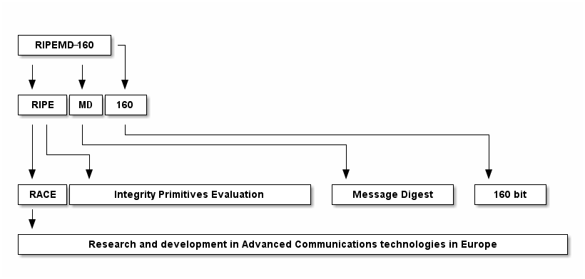
The RIPEMD-160 secure hash function may be best known these days for its role as part of the implementation of Bitcoin. I’ve wondered what “RIPEMD” stands for, and today I stumbled on an explanation [1]:

“RIPEMD” stands for “RIPE Message Digest,” where “RIPE” stands for “RACE Integrity Primitives Evaluation” and where “RACE” stands for “Research and Development in Advanced Communications Technologies in Europe”—a nice example of a recursive abbreviation.

This deserves a diagram:

I created the diagram above with DITAA.

Related posts

[1] Introduction to Cryptography with Open-Source Software by Alasdair McAndrew. CRC Press. 2011

Time dilation in SF and GPS

I’m reading Voyage to Alpha Centauri and ran into a question about relativity. The book says in one place that their ship is moving a 56.7% of the speed of light, and in another place it says that time moves about 20% slower for them relative to folks on Earth. Are those two statements consistent?

It wouldn’t bother me if they weren’t consistent. I ordinarily wouldn’t bother to check such things. But I remember looking into time dilation before and being surprised how little effect velocity has until you get very close to the speed of light. I couldn’t decide whether the relativistic effect in the novel sounded too large or too small.

If a stationary observer is watching a clock moving at velocity v, during one second of the observer’s time,

\sqrt{1 - \frac{v^2}{c^2}}

seconds will have elapsed on the moving clock.

Even at 20% of the speed of light, the moving clock only appears to slow down by about 2%.

If, as in the novel, a spaceship is moving at 56.7% of the speed of light, then for every second an Earth-bound observer experiences, someone on the ship will experience √(1 − 0.567²) = 0.82 seconds. So time would run about 20% slower on the ship, as the novel says.

The author must have either done this calculation or asked someone to do it for him. I had a science fiction author ask me for something a while back, though I can’t remember right now what it was.

Small velocities

You can expand the expression above in a Taylor series to get

\sqrt{1 - \frac{v^2}{c^2}} = 1 -\frac{v^2}{2c^2} -\frac{v^4}{8c^4} + \cdots

and so velocities much smaller than the speed of light, the effect of time dilation is 0.5 v²/c², a quadratic function of velocity. You can use this to confirm the comment above that when v/c = 0.2, the effect of time dilation is about 2%.

GPS satellites travel at about 14,000 km/hour, and so the effect of time dilation is on the order of 1 part in 1010. This would seem insignificant, except it amounts to milliseconds per year, and so it does make a practical difference.

For something moving 100 times slower, like a car, time dilation would be 10,000 times smaller. So time in a car driving at 90 miles per hour slows down by one part in 1014 relative to a stationary observer.

Tape measures

The math in the section above is essentially the same as the math in the post explaining why it doesn’t matter much if a tape measure does run exactly straight when measuring a large distance. They both expand an expression derived from the Pythagorean theorem in a Taylor series.