Evaluating and lowering AI hallucination cost

AI models hallucinate, and always will [1]. In some sense this is nothing new: everything has an error rate. But what is new is the nature of AI errors. The output of an AI is plausible by construction [2], and so errors can look reasonable even when they’re wrong. For example, if you ask for the capital city of Illinois, an AI might err by saying Chicago, but it wouldn’t say Seattle.

You need to decide two things when evaluating whether to use an AI for a task: the cost of errors and the cost of validation.

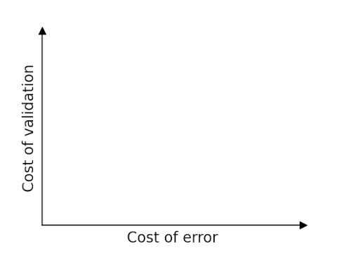
Cost of error on horizontal axis, cost of validation on vertical axis

Image generation is an ideal task for AIs because the consequences of an error are usually low. And validation is almost effortless: if an image looks OK, it’s OK. So imagine generation is in the bottom left corner of the image above.

Text-to-speech is a little more interesting to evaluate. The consequences of an error depend on user expectations. Someone may be mildly annoyed when a computer makes an error reading an email out loud, but the same person may angry if he thought he was talking to a human and discovers he’s been talking to a machine.

Validating text-to-speech requires a human to listen to the audio. This doesn’t require much effort, though the cost might be too much in some contexts. (I’m in the middle of an AI-narrated book and wondering why the producer didn’t go to the effort of fixing the pronunciation errors. The print version of the book has high production quality, but not as much effort went into the audio.) So I’d say text-to-speech is somewhere in the bottom half of the graph, but the horizontal location depends on expectations.

Code generation could be anywhere on the graph, depending on who is generating the code and what the code is being used for. If an experienced programmer is asking AI to generate code that in principle he could have written, then it should be fairly easy to find and fix errors. But it’s not a good idea for a non-programmer to generate code for a safety-critical system.

Mitigating risks and costs

The place you don’t want to be is up and to the right: errors are consequential and validation is expensive. If that’s where your problem lies, then you want to either mitigate the consequences of errors or reduce the cost of validation.

This is something my consultancy helps clients with. We find ways to identify errors and to mitigate the impact of inevitable errors that slip through.

If you’d like help moving down and to the left, lowering the cost of errors and the cost of validation, let’s set up a meeting to discuss how we can help.

LET’S TALK

[1] LLMs have billions of parameters, pushing a trillion. But as large as the parameter space is, the space of potential prompts is far larger, and so the parameters do not contain enough information to respond completely accurately to every possible prompt.

[2] LLMs predict the word that is likely to come next given the words produced so far. In that sense, the output is always reasonable. If an output does not appear reasonable to a human, it is because the human has more context.

Experiences with Nvidia

Our team started working within Nvidia in early 2009 at the beginning of the ORNL Titan project. Our Nvidia contacts dealt with applications, libraries, programming environment and performance optimization. First impressions were that their technical stance on issues was very reasonable. One obscure example: in a C++ CUDA kernel were you allowed to use “enums,” and the answer would be, of course, yes, we would allow that. This was unlike some other companies that might have odd and cumbersome programming restrictions in their parallel programming models (though by now this has become a harder problem for Nvidia since there are so many software products a user might want to interoperate).

Another example, with a colleague at Nvidia on the C++ standards committee, to whom I mentioned, it might be too early to lock this certain feature design into the standard since hardware designs are still rapidly changing. His response was, Oh, yes, we think exactly the same thing. So in short, their software judgments and decisions generally seem to be well thought out, reasonable and well informed. It sounds simple, but it is amazing how many companies have gotten this wrong.

Nvidia has made good strategic decisions. In the 2013 time frame, Intel was becoming a competitive threat with the Xeon Phi processor. Intel was several times larger than Nvidia with huge market dominance. In response, Nvidia formed a partnership with IBM–itself several times larger than Intel at the time. This came to fruition in the ORNL Summit system in 2018. In the meantime, the Xeon Phi’s OpenMP programming model, though standards-based, turned out to be difficult to write optimized code for, and Nvidia CUDA captured market share dominance of accelerated user software. Intel eventually dropped the Xeon Phi product line.

In the early 2000s, Nvidia went all-in on CUDA. I’ve heard some project teams say they would never use CUDA, because it is nonstandard and too low-level. Many have turned back on this decision. Of course, it is often possible to write an abstraction layer on top of CUDA to make it easier to use and maintain. Also newer programming models like Kokkos can be helpful.

Nvidia also made a prescient decision early to bet big on AI. A little later they decided to go all in on developing a huge number of software libraries is to enable access to many new markets. A huge moat. AMD is trying hard to improve their software processes and catch up.

On the downside, Nvidia high prices are upsetting to many, from gamers to buyers of the world’s largest HPC systems. Competition from AMD and others is a good thing.

And Nvidia marketing speak is sometimes confusing. A comparison was once made claiming that a four GPU system was more powerful than one of the world’s top CPU-only supercomputers on a very specific science problem. I’d like to see the details of that comparison. Also, different figures are being given on how long it took to stand up xAI’s Colossus supercomputer, from 19 days to 122 days. One has to dig a little to find out what these figures mean. Also it was widely reported last year that the GB200 NVL72 GPU was “30 times faster” than H100, but this only refers to certain operations, not key performance measures like flops per watt.

Those are my takes. For more perspectives, see Tae Kim’s excellent book, The Nvidia Way, or this interview.

Thoughts on Nvidia? Please leave in the comments.


Scientific papers: innovation … or imitation?

Sometimes a paper comes out that has the seeds of a great idea that could lead to a whole new line of pioneering research. But, instead, nothing much happens, except imitative works that do not push the core idea forward at all.

For example the McCulloch Pitts paper from 1943 showed how neural networks could represent arbitrary logical or Boolean expressions of a certain class. The paper was well-received at the time, brilliantly executed by co-authors with diverse expertise in neuroscience, logic and computing. Had its significance been fully grasped, this paper might have, at least notionally, formed a unifying conceptual bridge between the two nascent schools of connectionism and symbolic AI (one can at least hope). But instead, the heated conflict in viewpoints in the field has persisted, even to this day.

Another example is George Miller’s 7 +/- 2 paper. This famous result showed humans are able to hold only a small number of pieces of information in mind at the same time while reasoning.  This paper was important not just for the specific result, but for the breakthrough in methodology using rigorous experimental noninvasive methods to discover how human thinking works—a topic we know so little about, even today. However, the followup papers by others, for the most part, only extended or expanded on the specific finding in very minor ways. [1] Thankfully, Miller’s approach did eventually gain influence in more subtle ways.

Of course it’s natural from the incentive structures of publishing that many papers would be primarily derivative rather than original. It’s not a bad thing that, when a pioneering paper comes out, others very quickly write rejoinder papers containing evaluations or minor tweaks of the original result. Not bad, but sometimes we miss the larger implications of the original result and get lost in the details.

Another challenge is stovepiping—we get stuck in our narrow swim lanes for our specific fields and camps of research. [2] We don’t see the broader implications, such as connections and commonalities across fields that could lead to fruitful new directions.

Thankfully, at least to some extent current research in AI shows some mix of both innovation and imitation. Inspired in part by the accelerationist mindset, many new papers appear every day, some with significant new findings and others that are more modest riffs on previous papers.

Notes

[1] Following this line of research on human thought processes could be worthwhile for various reasons. For example, some papers in linguistics state that Chomsky‘s vision for a universal grammar is misguided because the common patterns in human language are entirely explainable by the processing limitations of the human mind. But this claim is made with no justification or methodological rigor of any kind. If I claimed a CPU performs vector addition or atomic operations efficiently because of “the capabilities of the processor,” I would need to provide some supporting evidence, for example, documenting that the CPU has vector processing units or specialized hardware for atomics. The assertions about language structure being shaped by the human mental processing faculty is just an empty truism, unless supported by some amount of scientific rigor and free of the common fallacies of statistical reasoning.

[2] I recently read a paper in linguistics with apparent promise, but the paper totally misconstrued the relationship between Shannon entropy and Kolmogorov complexity. Sadly this paper passed review in a linguistic journal, but if it had had a mathematically inclined reviewer, the problem would have been caught and fixed.


Why do LLMs have emergent properties?

Large language models display emergence behaviors: when the parameter count is scaled to a certain value, suddenly the LLM is capable of performing a new task not possible at a smaller size. Some say the abruptness of this change is merely a spurious artifact of how it is measured. Even so, many would like to understand, predict, and even facilitate the emergence of these capabilities.

The following is not a mathematical proof , but a plausibility argument as to why such behavior should not be surprising, and a possible mechanism. I’ll start with simple cases and work up to more complex ones.

In nature

An obvious point. Emergence is ubiquitous in nature. Ice near the freezing point that is slightly heated suddenly becomes drinkable (phase change). An undrivable car with three wheels gets a fourth wheel and is suddenly drivable. Nonlinearity exists in nature.

In machine learning

A simple example: consider fitting N arbitrary points in one dimension with linear regression using monomials. For a basis up to degree less than N-1, for most possible sets of data points (excluding “special” cases like collinear), the regression error will be non-zero, and reciprocally, the accuracy will be some finite value. Increase the number of monomials (parameter count) to N-1, and suddenly the error drops to zero, and accuracy jumps to infinity.

When using k-means clustering, if one has n clusters and runs k-means clustering with K<N cluster centers, the error will be significant, but when K=N, suddenly the cluster centers can model all clusters well, and the error drops dramatically.

In algorithms

Consider all Boolean circuits composed from some fixed logically complete set of gate types. Now consider the goal of constructing a Boolean circuit that takes a single byte representing the integer N and increments it to N+1, modulo 256 (8 bits input, 8 bits output). Clearly, such a circuit exists, for example, the standard chain of 1-bit add-and-carry circuits. Note one can in principle enumerate all possible circuits of finite gate count. It is manifest that an integer K>0 exists for which no circuit with less than K gates solves the problem but there exists a circuit with K gates that does. The standard chain of 8 1-bit adders might be such a minimizer, or maybe the optimal circuit is more exotic (for example see here, though this method is not guaranteed to compute a minimizer).

One would thus see this capability potentially emerge as soon as one reaches a gate budget of K gates. Now, one could argue that for a smaller gate budget, a partial result might be possible, for example, incrementing any 7-bit number—so the increase in capability is continuous, not emergent or wholly new. However, if all you care about is correctly incrementing any byte (for example, for manipulating ASCII text), then it’s all or nothing; there’s no partial credit. Even so, the gate budget required for incrementing 8 bits compared to only 7-bit integers is only slightly higher, but this minor increase in gate count actually doubles the quantity of integers that can be incremented, which might be perceived as a surprising, unexpected (emergent) jump.

In LLMs

The parameter count of an LLM defines a certain bit budget. This bit budget must be spread across many, many tasks the final LLM will be capable of, as defined by the architecture and the training process (in particular, the specific mix of training data). These tasks are implemented as “algorithms” (circuits) within the LLM. The algorithms are mixed together and (to some extent) overlap in a complex way that is difficult to analyze.

Suppose one of these desired capabilities is some task X. Suppose all possible input/output pairs for this operation are represented in the training data (or, maybe not—maybe some parts of the algorithm can be interpolated from the training data). The LLM is trained with SGD, typically with 2-norm minimization. The unit ball in the 2-norm is a sphere in high dimensional space. Thus “all directions” of the loss are pressed down equally by the minimization process—which is to say, the LLM is optimized on all the inputs for many, many tasks, not just task X. The limited parameter bit budget must be spread across many, many other tasks the LLM must be trained to do. As LLMs of increasing size are trained, at some point enough parameter bits in the budget will be allocatable to represent a fully accurate algorithm for task X, and at this point the substantially accurate capability to do “task X” will be perceivable—“suddenly.”

Task X could be the 8-bit incrementer, which from an optimal circuit standpoint would manifest emergence, as described above. However, due to the weakness of the SGD training methodology and possibly the architecture, there is evidence that LLM training does not learn optimal arithmetic circuits at all but instead does arithmetic by a “bag of heuristics” (which incidentally really is, itself, an algorithm, albeit a piecemeal one). In this case, gradually adding more and more heuristics might be perceived to increase the number of correct answers in a somewhat more incremental way, to be sure. However, this approach is not scalable—to perform accurate arithmetic for any number of digits, if one does not use an exact arithmetic algorithm or circuit, one must use increasingly more heuristics to increase coverage to try to capture all possible inputs accurately. And still, transitioning from an approximate to an exact 8-bit incrementer might in practice be perceived as an abrupt new capability, albeit a small one for this example.

One could alternatively consider tool use (for example, a calculator function that is external to the LLM proper), but then a new tool must be written for every new task, and the LLM needs to understand how to use the tool. (Maybe at some point LLMs will know how to write and use their own algorithmic tools?)

Predicting emergence

The real question is how can we predict when a new LLM will achieve some new capability X. For example, X = “Write a short story that resonates with the social mood of the present time and is a runaway hit” (and do the same thing again once a year based on new data, indefinitely into the future without failure). We don’t know an “algorithm” for this, and we can’t even begin to guess the required parameter budget or the training data needed. That’s the point of using an LLM—its training internally “discovers” new, never seen before algorithms from data that would be difficult for humans to formulate or express from first principles. Perhaps there is some indirect way of predicting the emergence of such X, but it doesn’t seem obvious on the face of it how to predict this directly.

Conclusion

Based on these examples, it would seem not at all surprising for LLMs to exhibit emergent behaviors, though in our experience our encounter with them may be startling. Predicting them may be possible to a limited extent but for the general case seems really hard.

Do you have any thoughts? If so, please leave them in the comments.

Looking at Your Data

What to do first after scoping out and starting a data science project?

I’ve started an unsupervised learning project based on textual data. The first thing I like to do is actually look at the data. Is it noisy? What are the features—complex feature engineering needed? How heterogeneous? What generalization and overfitting challenges?

Analysis can take many forms: actually looking at the numbers, using visualization tools, Excel spreadsheet, Jupyter notebooks with Matplotlib, computing various statistics on the whole dataset or portions of it.

Some may believe this is not important. Just throw a barrage of classification or regression methods at the data, treat the data as a black box. Of course testing on a suite of ML methods is not a bad thing. But I can’t imagine not using every avenue available, including looking at the data. I’m certainly not alone in this view (see for example here, here and here).

I spent a few hours developing a simple custom data viewer for my problem that colored different parts of the textual data to give insight as to what was going on. I used ChatGPT to develop parts of this tool; some of it was incorrect and needed fixing, but having at least a draft of the code definitely saved time. Seeing the actual data in person was insightful and generated ideas for solving the problem.

While inspecting the data can help identify issues, it also risks biasing the modeling process by imposing assumptions that a flexible model might otherwise uncover on its own. One must also beware of data leakage. That being said—in general I think understanding as much as you can about the data is not a bad thing.

Lessons Learned With the Z3 SAT/SMT Solver

Community best practices are useful for helping use a software product more effectively. I’ve just completed a small project using the Z3 solver. Here are some things I’ve learned:

  • My project involves an optimization problem: for a subset of Boolean variables, maximize the count of how many are true. My specific problem is solved much faster with Z3 by converting to a decision problem: set up a base problem to solve for the count being at least a certain fixed number, and iterate using bisection search to find the highest number satisfied. Bisection has been used for this problem before. Also, certain methods may possibly reduce the number of bisection steps.
  • Using Z3  “tactics” can greatly speed up the solve process. I found a good combination of tactics by trial and error, guided in part by the descriptions of the tactics. ChatGPT was of some help in finding good selections to try. An interesting paper discusses use of Monte Carlo tree search to define a good chain of tactics. The branching factor here is high, perhaps around 1000, though there are some redundancies in this number. Training multi-step MCTS might be expensive, but doing this once to get a good static chain of tactics might be worthwhile.
  • The strength of Z3 is in its extremely broad functionality, more so than its raw compute performance. It would be a daunting task for the Z3 team to fully optimize every possible solve option. I examined some of the SMT solver competitions to find faster codes. CVC5 on one case I tried was about twice as fast as Z3; I’ve seen similar reports in the literature. Presently I don’t find it worth the switching costs to use CVC5. One approach might be to use the very capable tactics engine of Z3 and pass the resulting modified problem to CVC5.
  • The specific formulation of the problem can make a big difference in solver performance. I’ve already seen this in the area of iterative linear solvers, for example diagonal matrix scaling can dramatically help (conjugate gradients) or hurt (multigrid) solver performance. Same thing here. Hence the huge importance in good “preprocessing“ for SAT/SMT solvers. One could wish the solver could handle all this automatically without user intervention. However, these powerful tools must be brandished very carefully for maximum effect.
  • Generally, one should move as much of the problem outside of the solver as possible, since the solver is the long pole in the tent in terms of scalability. For example if there is a Z3 integer that must be limited to a certain range and additionally some values in the interval must be blacklisted, it’s better, if possible, to compress all of the valid values into a single interval, to make testing for validity simpler in the Z3 code.
  • Along these lines: the Z3 tactics for propagating constants are not perfect; thus it can help to manually propagate constants (though this unfortunately makes the code more messy). This propagation can also sometimes allow for removal of unneeded constraints, further speeding up performance. Relatedly, some intriguing work by Benjamin Mikek shows how one can use the LLVM code optimizer to optimize the SMT problem in a way that is complementary to Z3 tactics, achieving significant speedup (for more info see here, here and here). I haven’t tried this but it seems promising.
  • CPU threading does not work for my case (Z3 Python, macOS). Perfect parallelization of SAT and SMP is an unsolved (and perhaps in some sense not fully solvable) problem. One can naïvely parallelize bisection search by converting to trisection, etc., but this does not give perfect speedup (specif., log(P) speedup on P threads). Improvements to parallel bisection in some cases may be possible. Recent work by Armin Biere and colleagues looks promising; as I read it, near perfect speedup up to eight threads (at least for some problems).
  • Some of the main developers of Z3 are on Stack Overflow and have been active in the past answering questions. This seems very useful.

Resources like Handbook of Satisfiability and the proceedings of various SAT/SMT conferences seem helpful. More information on best practices for non-expert practitioners would be a great help to the community. If you know of any good resources, please share in the comments.

Grokking the James Bond chord

The last chord of the James Bond theme is known as the James Bond chord. If you’ve ever seen a Bond movie, you’ll recognize it. Here’s a quick video showing how to play it on guitar.

I tried asking Grok 3 to generate some LilyPond code for sheet music a few days ago. LilyPond is pretty obscure as programming languages go—it’s not like asking for Python code—so I was skeptical, but Grok did well.

This afternoon I asked Grok to create sheet music for the James Bond chord. Specifically, I asked

  1. What is the “James Bond chord”?
  2. Create sheet music for the James Bond chord using Lilypond.
  3. Move the chord up an octave.

Here’s the output of each step.

What is the chord?

According to Grok,

The “James Bond chord” is a distinctive musical chord famously associated with the James Bond film franchise. It’s not just a single chord but rather a specific voicing and progression that evokes a sense of mystery, danger, and sophistication—perfectly matching the suave spy’s persona. Officially, it’s often identified as an E minor major 9 chord (EmMaj9), though its exact interpretation can vary slightly depending on the context.

The chord was first introduced by composer Monty Norman in the “James Bond Theme” for Dr. No (1962), arranged by John Barry, whose orchestration gave it its iconic swagger. …

First output

Grok produced the following LilyPond code

\version "2.22.0"

\score {
  \new Staff {
    \clef treble
    \key c \major % Default key, no sharps/flats; we'll specify accidentals manually
    \time 4/4
     <e g b dis' fis'>1 % EmMaj9 chord: E G B D# F#
  }
  \layout {}
  \midi {}
}

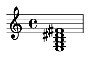
When compiled this gave the following music.

Grok also produce a MIDI file.

Second output

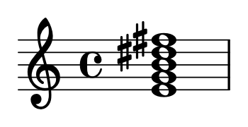
I wanted to move the chord up an octave for aesthetic reasons, putting the notes inside the staff. Grok complied, changing one line in the code, essentially adding an extra prime mark after each note.

<e' g' b' dis'' fis''>1 % EmMaj9 chord moved up an octave: E' G' B' D#'' F#''

This compiled to the following music.

Problems and prospects

Grok’s not perfect. In another experiment it produced code that wouldn’t compile. But when I told Grok that the code didn’t compile and asked it to try again, it worked.

I tried to remove the time signature, the C symbol. I asked Grok to remove it, and it did not. I asked Grok “How do you get LilyPond to produce music without a time signature?” and it told me two ways, neither of which worked.

I’ve used LilyPond occasionally for years, not to produce full sheets of music but to produce little fragments for blog posts. I’ve always found it a bit mysterious, in part because I jumped in and used it as needed without studying it systematically. There have been times when I thought about including some music notation in a blog post and didn’t want to go to the effort of using LilyPond (or rather the effort of debugging LilyPond if what I tried didn’t work). I may go to the effort more often now that I have a fairly reliable code generator.

Posts using LilyPond

Practical consequences of tokenization details

I recently ran across the article Something weird is happening with LLMs and chess. One of the things it mentions is how the a minor variation in a prompt can have a large impact on the ability of an LLM to play chess.

One extremely strange thing I noticed was that if I gave a prompt like “1. e4 e5 2. ” (with a space at the end), the open models would play much, much worse than if I gave a prompt like “1 e4 e5 2.” (without a space) and let the model generate the space itself. Huh?

The author goes on to explain that tokenization probably explains the difference. The intent is to get the LLM to predict the next move, but the extra space confuses the model because it is tokenized differently than the spaces in front of the e’s. The trailing space is tokenized as an individual character, but the spaces in front of the e’s are tokenized with the e’s. I wrote about this a couple days ago in the post The difference between tokens and words.

For example, ChatGPT will tokenize “hello world” as [15339, 1917] and “world hello” as [14957, 24748]. The difference is that the first string is parsed as “hello” and ” world” while the latter is parsed as “world” and ” hello”. Note the spaces attached to the second word in each case.

The previous post was about how ChatGPT tokenizes individual Unicode characters. It mentions UTF-16, which is itself an example of how tokenization matters. The string “UTF-16” it will be represented by three tokens, one each for “UTF”, “-“, and “16”. But the string “UTF16” will be represented by two tokens, one for “UTF” and one for “16”. The string “UTF16” might be more likely to be interpreted as a unit, a Unicode encoding.

ChatGPT tokens and Unicode

I mentioned in the previous post that not every Unicode character corresponds to a token in ChatGPT. Specifically I’m looking at gpt-3.5-turbo in tiktoken. There are 100,256 possible tokens and 155,063 Unicode characters, so the pigeon hole principle says not every character corresponds to a token.

I was curious about the relationship between tokens and Unicode so I looked into it a little further.

Low codes

The Unicode characters U+D800 through U+DFFF all map to a single token, 5809. This is because these are not really characters per se but “surrogates,” code points that are used in pairs to represent other code points [1]. They don’t make sense in isolation.

The character U+FFFD, the replacement character �, also corresponds to 5809. It’s also not a character per se but a way to signal that another character is not valid.

Aside from the surrogates and the replacement characters, every Unicode character in the BMP, characters up to U+FFFF, has a unique representation in tokens. However, most require two or three tokens. For example, the snowman character ☃ is represented by two tokens: [18107, 225].

Note that this discussion is about single characters, not words. As the previous post describes, many words are tokenized as entire words, or broken down into units larger than single characters.

High codes

The rest of the Unicode characters, those outside the BMP, all have unique token representations. Of these, 3,404 are represented by a single token, but the rest require 2, 3, or 4 tokens. The rocket emoji, U+1F680, for example, is represented by three tokens: [9468, 248, 222].

Rocket U+1F680 [9468, 248, 222]

[1] Unicode was originally limited to 16 bits, and UFT-16 represented each character with a 16-bit integer. When Unicode expanded to beyond 216 characters, UTF-16 used pairs of surrogates, one high surrogate and one low surrogate, to represent code points higher than U+FFFF.

The difference between tokens and words

Large language models operate on tokens, not words, though tokens roughly correspond to words.

A list of words would not be practical. There is no definitive list of all English words, much less all words in all languages. Still, tokens correspond roughly to words, while being more flexible.

Words are typically turned into tokens using BPE (byte pair encoding). There are multiple implementations of this algorithm, giving different tokenizations. Here I use the tokenizer gpt-3.5-turbo used in GPT 3.5 and 4.

Hello world!

If we look at the sentence “Hello world!” we see that it turns into three tokens: 9906, 1917, and 0. These correspond to “Hello”, ” world”, and “!”.

In this example, each token corresponds to a word or punctuation mark, but there’s a little more going on. It is true that 0 is simply the token for the exclamation mark—we’ll explain why in a moment—it’s not quite true to say 9906 is the token for “hello” and 1917 is the token for “world”.

Many to one

In fact 1917 is the token for ” world”. Note the leading space. The token 1917 represents the word “world,” not capitalized and not at the beginning of a sentence. At the beginning of a sentence, “World” would be tokenized as 10343. So one word may correspond to several different tokens, depending on how the word is used.

One to many

It’s also true that a word may be broken into several tokens. Consider the sentence “Chuck Mangione plays the flugelhorn.” This sentence turns into 9 tokens, corresponding to

“Chuck”, “Mang”, “ione”, ” plays”, ” fl”, “ug”, “el”, “horn”, “.”

So while there is a token for the common name “Chuck”, there is no token for the less common name “Mangione”. And while there is a single token for ” trumpet” there is no token for the less common “flugelhorn.”

Characters

The tokenizer will break words down as far as necessary to represent them, down to single letters if need be.

Each ASCII character can be represented as a token, as well as many Unicode characters. (There are 100256 total tokens, but currently 154,998 Unicode characters, so not all Unicode characters can be represented as tokens.)

Update: The next post dives into the details of how Unicode characters are handled.

The first 31 ASCII characters are non-printable control characters, and ASCII character 32 is a space. So exclamation point is the first printable, non-space character, with ASCII code 33. The rest of the printable ASCII characters are tokenized as their ASCII value minus 33. So, for example, the letter A, ASCII 65, is tokenized as 65 − 33 = 32.

Tokenizing a dictionary

I ran every line of the american-english word list on my Linux box through the tokenizer, excluding possessives. There are 6,015 words that correspond to a single token, 37,012 that require two tokens, 26,283 that require three tokens, and so on. The maximum was a single word, netzahualcoyotl, that required 8 tokens.

The 6,015 words that correspond to a single token are the most common words in English, and so quite often a token does represent a word. (And maybe a little more, such as whether the word is capitalized.)