About half of children are boys and half are girls, but that doesn’t mean that every couple is equally likely to have a boy or a girl each time they conceive a child. And evidence suggests that indeed the probability of conceiving a girl varies per couple.
I will simplify things for this post and look at a hypothetical situation abstracting away the complications of biology. This post fills in the technical details of a thread I posted on Twitter this morning.
Suppose the probability p that a couple will have a baby girl has a some distribution centered at 0.5 and symmetric about that point. Then half of all births on the planet will be girls, but that doesn’t mean that a particular couple is equally likely to have a boy or a girl.
How could you tell the difference empirically? You couldn’t if every family had one child. But suppose you studied all families with four children, for example. You’d expect 1 in 16 such families to have all boys, and 1 in 16 families to have all girls. If the proportions are higher than that, and they are, then that suggests that the distribution on p, the probability of a couple having a girl, is not constant.
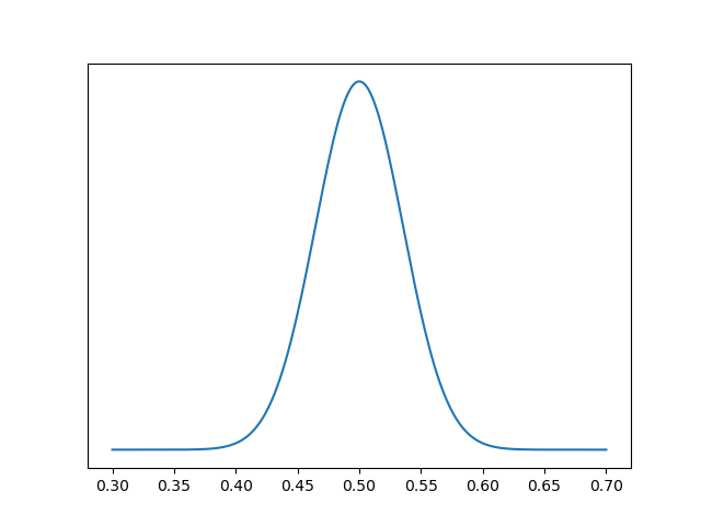
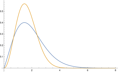
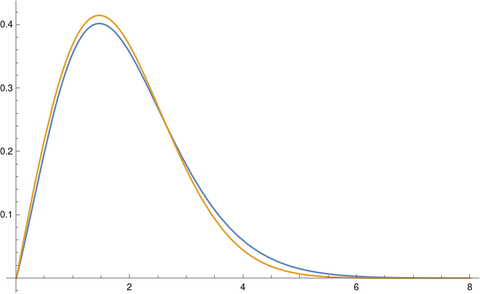
Suppose the probability of a couple having girls has a beta(a, b) distribution. We would expect a and b to be approximately equal, since about half of babies are girls, and we’d expect a and b to be large, i.e. for the distribution be fairly concentrated around 1/2. For example, here’s a plot with a = b = 100.
Then the probability distribution for the number of girls in a family of n children is given by a beta-binomial distribution with parameters n, a, and b. That is, the probability of x girls in a family of size n is given by
![]()
The mean of this distribution is na/(a+b). And so if a = b then the mean is n/2, half girls and half boys.
But the variance is more interesting. The variance is
![]()
The variance of a binomial, corresponding to a constant p, is np(1-p). In the equation above, p corresponds to a/(a+b), and (1-p) corresponds to b/(a+b). And there’s an extra term,
![]()
which is larger than 1 when n > 1. This says a beta binomial random variable always has more variance than the corresponding binomial distribution with the same mean.
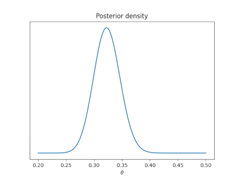
Now suppose a family has had n children, with g girls and n – g boys. Then the posterior predictive probability of a girl on the next birth is
![]()
If g = n/2 then this probability is 1/2. But if g > n/2 then the probability is greater than 1/2. And the smaller a and b are, the more the probability exceeds 1/2.
The binomial model is the limit of the beta-binomial model as a and b go to infinity (proportionately). In the limit, the probability above equals a/(a+b), independent of g and n.


