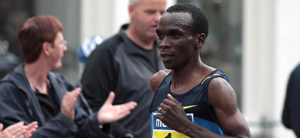
I ran across the image below [1] when I was searching for something else, and it made me think of a few issues in data privacy.
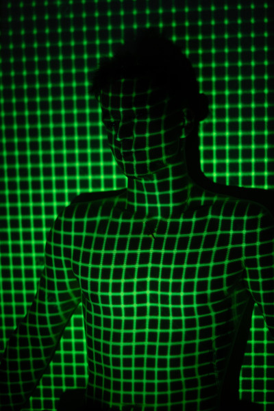
The green lights cut across the man’s body like tomographic imaging. No one of these green lines would be identifiable, but maybe the combination of the lines is.
We can tell it’s a young man in the image, someone in good shape. But is this image identifiable?
It’s identifiable to the photographer. It’s identifiable to the person in the photo.
If hundreds of men were photographed under similar circumstances, and we knew who those men were, we could probably determine which of them is in this particular photo.
The identifiability of the photo depends on context. The HIPAA Privacy Rule acknowledges that the risk of identification of individuals in a data set depends on who is receiving the data and what information the recipient could reasonably combine the data with. The NSA could probably tell who the person in the photo is; I cannot.
Making photographs like this available is not a good idea if you want to protect privacy, even if its debatable whether the person in the photo can be identified. Other people photographed under the same circumstances might be easier to identify.
Differential privacy takes a more conservative approach. Differential privacy advocates argue that deidentification procedures should not depend on what the recipient knows. We can never be certain what another person does or doesn’t know, or what they might come to know in the future.
Conventional approaches to privacy consider some data more identifiable than other data. Your phone number and your lab test results from a particular time and place are both unique, but the former is readily available public information and the latter is not. Differential privacy purists would say both kinds of data should be treated identically. A Bayesian approach might be to say we need to multiply each risk by a prior probability: the probability of an intruder looking up your phone number is substantially greater than the probability of the intruder accessing your medical records.
Some differential privacy practitioners make compromises, agreeing that not all data is equally sensitive. Purists decry this as irresponsible. But if the only alternatives are pure differential privacy and traditional approaches, many clients will choose the latter, even though an impure approach to differential privacy would have provided better privacy protection.
[1] Photo by Caspian Dahlström on Unsplash


