Simple derivation of exponential approximation

I was watching one of Brian Douglas’ videos on control theory (Discrete Control #5) and ran into a simple derivation of an approximation I presented earlier.

Back in April I wrote several post on simple approximations for log, exp, etc. In this post I gave an approximation for the exponential function:

\exp(x) \approx \frac{2 + x}{2 - x}

The control theory video arrives at the same approximation as follows.

\begin{align*} \exp(x) &= \exp(x/2)\, \exp(x/2) \\ &= \frac{\exp(x/2)}{\exp(-x/2)} \\ &\approx \frac{1 + x/2}{1 - x/2} \\ &= \frac{2 + x}{2-x} \end{align*}

As I believe I’ve suggested before here, in a derivation like the one above, where you have mostly equalities and one or two approximations, pay special attention to the approximation steps. The approximation step above uses a first order Taylor approximation in the numerator and denominator.

The plot below shows that the approximation above (the bilinear approximation) is more accurate than doing a single Taylor approximation, approximating exp(x) by 1 + x (linear approximation).

exp, linear approx, bilinear approx

Here’s a plot focusing on the error in the bilinear and linear approximations.

error in linear and bilinear approximations to exp

The bilinear approximation is hard to tell from 0 in the plot above for x up to 0.5.

The derivation above is simple, but why is the result so good? An explanation in terms of Padé approximation is given here.

Upper case, lower case, title case

Converting text to all upper case or all lower case is a fairly common task.

One way to convert text to upper case would be to use the tr utility to replace the letters a through z with the letters A through Z. For example,

    $ echo Now is the time | tr '[a-z]' '[A-Z]'
    NOW IS THE TIME

You could convert to lower case by reversing the arguments to tr.

The approach above works if your text consists of only unadorned Roman letters. But it wouldn’t work, for example, if you gave it a jalapeño or π:

    $ echo jalapeño π | tr '[a-z]' '[A-Z]'
    JALAPEñO π

Using the character classes [:lower:] and [:upper:] won’t help either.

Tussling with Unicode

One alternative would be to use the uc command from the Unicode::Tussle package [1] I mentioned a few days ago. There’s also a lc counterpart, and a tc for title case. These utilities handle far more than Roman letters.

    $ echo jalapeño π | uc
    JALAPEÑO Π

Unicode capitalization rules are a black hole, but we’ll just look at one example and turn around quickly before we cross the event horizon.

Suppose you want to send all the letters in the Greek word σόφος to upper case.

    $ echo σόφος | uc
    ΣΌΦΟΣ

Greek has two lower case forms of sigma: ς at the end of a word and σ everywhere else. But there’s only one upper case sigma, so both get mapped to Σ. This means that if we convert the text to upper case and then to lower case, we won’t end up exactly where we started.

    $ echo σόφος | uc | lc
    σόφοσ

Note that the lc program chose σ as the lower case of Σ and didn’t take into account that it was at the end of a word.

Related posts

[1] “Tussle” is an acronym for Tom [Christiansen]’s Unicode Scripts So Life is Easier.

Continued fraction from entropy source testing

NIST publication 800-90B, Recommendations for the Entropy Sources Used for Random Bit Generation, contains an interesting continued fraction.

Define a function

F\left(\frac{1}{z}\right) = \Gamma(3,z) z^{-3} e^z

where

\Gamma(a, b) = \int_b^\infty t^{a-1} e^{-t} \, dt

is the incomplete gamma function.

NIST 800-90B gives [1] a continued fraction implement F, but the continued fraction includes a parameter k for no apparent reason. NIST cites a paper that in turn cites Abramowitz and Stegun formula 6.5.31.

It appears that the k in NIST 800-90B corresponds to a − 1 in A&S 6.5.31, where a is the first argument to the incomplete gamma function and the exponent on 1/z, and so a = 3.

The continued fraction in A&S is

\cfrac{1}{z+\cfrac{1-a}{1+\cfrac{1}{z+\cfrac{2-a}{1+ \cfrac{2}{z +\ddots}}}}}

However, it’s not entirely clear how to fill in the dots. Apparently the denominators alternate between z and 1, but what about the numerators. The pattern we are give is

1, 1 − a, 1, 2 − a, 2

That’s as far as A&S goes. My initial guess was that we should ignore the 1 at the beginning of the series. In that case the rest of the series would be

3 − a, 3, 4 − a, 4, …

and that turns out to be right. If you don’t ignore the first 1, it can be hard to figure out how it fits into the pattern (because it doesn’t!).

How many terms of the continued fraction do we need? It depends on the size of the argument z. For large z, say z > 4, the terms shown above give a good approximation. But for smaller z, the approximation is terrible. For example, F(1) = 5, but the continued fraction evaluated at 1 gives −3/2.

The NIST paper requires evaluating F for values around 1, and it would take some work to figure out how far to carry the continued fraction before it is reliable in that range.

Related posts

[1] Why does NIST include a way to compute F? The incomplete gamma function is difficult to implement well and some mathematical libraries don’t include it. Having a stand-alone implementation of this function might make a testing program more self-contained.

Removing Unicode formatting

Several people responded to my previous post asserting that screen readers would not be able to read text formatted via Unicode variants. Maybe some screen readers can’t handle this, but there’s no reason they couldn’t.

Before I go any further, I’d like to repeat my disclaimer from the previous post:

It’s a dirty hack, and I’d recommend not overdoing it. But it could come in handy occasionally. On the other hand, some people may not see what you intend them to see.

This formatting is gimmicky and there are reasons to only use it sparingly or not at all. But I don’t see why screen readers need to be stumped by it.

In the example below, I format the text “The quick brown fox” by running it through unifont as in the previous post.

If we pipe the output through unidecode then we mostly recover the original text. (I wrote about unidecode here.)

    $ unifont The quick brown fox | unidecode 

            Double-Struck: The quick brown fox
                Monospace: The quick brown fox
               Sans-Serif: The quick brown fox
        Sans-Serif Italic: The quick brown fox
          Sans-Serif Bold: The quick brown fox
   Sans-Serif Bold Italic: The quick brown fox
                   Script: T he quick brown fox
                   Italic: The quick brown fox
                     Bold: The quick brown fox
              Bold Italic: The quick brown fox
                  Fraktur: T he quick brown fox
             Bold Fraktur: T he quick brown fox

The only problem is that sometimes there’s an extra space after capital letters. I don’t know whether this is a quirk of unifont or unidecode.

This isn’t perfect, but it’s a quick proof of concept that suggests this shouldn’t be a hard thing for a screen reader to do.

Maybe you don’t want to normalize Unicode characters this way all the time, but you could have some configuration option to only do this for Twitter, or to only do it for characters outside a certain character range.

How to format text in Twitter

Twitter does not directly provide support for formatting text in bold, italic, etc. But it does support Unicode characters [1], and so a hack to get around the formatting limitation is to replace letters with Unicode variants.

For example, you could tweet

How to include bold or italic text in a tweet.

I cheated in the line above, using bold and italic formatting rather than Unicode characters because some readers might not be able to read it.

Here’s a screenshot of the actual Unicode text in Emacs. You can see the text in the footnotes [2].

This is plain text. I have asked for the details on the ‘b’ in bold, and the bottom windows shows that it is not the common U+0062 for ‘b’ down in the ASCII range, but U+1D5EF up in the Supplementary Multilingual Plane. Similarly, the i in italic above is not U+0069 but U+1D456.

Here’s how the text appears in Twitter:

It’s a dirty hack, and I’d recommend not overdoing it. But it could come in handy occasionally. On the other hand, some people may not see what you intend them to see. Here’s a portion of a screenshot from an Android device:

How to include XXXX or XXXXXX test

As a very rough rule of thumb, characters with smaller Unicode values are more likely to display correctly everywhere. Math symbols like ∞ (U+221E) work everywhere as far as I know. I wouldn’t depend on any Unicode character above 0xFFFF.

Update: Several people have said this formatting poses a problem for speech readers. The next post explains why it shouldn’t. (Maybe it does cause a problem, but it wouldn’t have to.)

How to produce Unicode formatting

I produced the Unicode text above using the programs unifont and unisupers from the Perl module Unicode::Tussle. See this post for how to install the module. Here’s a screenshot of using these utilities from the command line.

To use unifont, type the text you’d like to format after the command. It then shows the text formatted several ways using Unicode characters. I typed “bold” and copied the bold version of the word. The text could be anything; it’s a coincidence that I gave it text that was also a format name. For example, I created the double-struck R and C above with the command

    unifont R C

The unisupers command does not take an argument but instead takes its input from standard input. So I hit return after the command name and then typed ‘n’ to get the superscript n.

Related posts

[1] Twitter supports Unicode characters, but there’s a question of whether readers will have fonts installed to display the characters. I wrote eight years ago about some symbols users were and were not likely to see, but my impression is that the situation has improved quite a bit since then.

[2] Here’s the actual text of the tweet:

How to include  or  text in a tweet.
Weierstrass function.
Im: ℂ -> ℝ
ℝⁿ -> ℝᵐ

(I pasted the text into my blogging software, but it looks like it is deleting the words “bold” and “italic.”)

Predator-Prey period

The Lotka-Volterra equations are a system of nonlinear differential equations for modeling a predator-prey ecosystem. After a suitable change of units the equations can be written in the form

\begin{align*} \frac{dx}{dt} &= \phantom{-}ax(y-1) \\ \frac{dy}{dt} &= -by(x-1) \end{align}

where ab = 1. Here x(t) is the population of prey at time t and y(t) is the population of predators. For example, maybe x represents rabbits and y represents foxes, or x represents Eloi and y represents Morlocks.

It is well known that the Lotka-Volterra equations have periodic solutions. It is not as well known that you can compute the period of a solution without having to first solve the system of equations.

This post will show how to compute the period of the system. First we’ll find the period by solving the equations for a few different initial conditions, then we’ll show how to directly compute the period from the system parameters.

Phase plot

Here is a plot of (x(t), y(t)) showing that the solutions are periodic.

Predator-prey phase plots for varying initial conditions

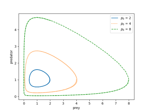
And here’s the Python code that made the plot above.

    import matplotlib.pyplot as plt
    import numpy as np
    from scipy.integrate import solve_ivp
    
    # Lotka-Volterra equations
    def lv(t, z, a, b):
        x, y = z
        return [a*x*(y-1), -b*y*(x-1)]
    
    begin, end = 0, 20
    t = np.linspace(begin, end, 300)
    
    styles = ["-", ":", "--"]
    prey_init = [2, 4, 8]
    a = 1.5
    b = 1/a
    
    for style, p0 in zip(styles, prey_init):
        sol = solve_ivp(lv, [begin, end], [p0, 1], t_eval=t, args=(a, b))
        plt.plot(sol.y[0], sol.y[1], style)
    
    plt.xlabel("prey")
    plt.ylabel("preditor")
    plt.legend([f"$p_0$ = {p0}" for p0 in prey_init])    

Note that the derivative of x is zero when y = 1. Since our initial condition sets y(0) = 1, we’re specifying the maximum value of x. (If our initial values of x were less than 1, we’d be specifying the minimum of x.)

Time plot

The components x and y have the same period, and that period depends on a and b, and on the initial conditions. The plot below shows how the period increases with x(0), which as we noted above is the maximum value of x.

Predator-prey solutions over time for varying initial conditions

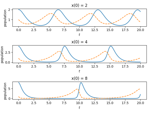
And here’s the code that made the plot.

    fig, ax = plt.subplots(3, 1)
    for i in range(3):
        sol = solve_ivp(lv, [begin, end], [prey_init[i], 1], t_eval=t, args=(a, b))
        ax[i].plot(t, sol.y[0], "-")
        ax[i].plot(t, sol.y[1], "--")    
        ax[i].set_xlabel("$t$")
        ax[i].set_ylabel("population")
        ax[i].set_title(f"x(0) = {prey_init[i]}")
    plt.tight_layout()

Finding the period

In [1] the author develops a way to compute the period of the system as a function of its parameters without solving the differential equations.

First, calculate an invariant h of the system:

h = b(x - \log(x) - 1) + a(y - \log(y) - 1)

Since this is an invariant we can evaluate it anywhere, so we evaluate it at the initial conditions.

Then the period only depends on a and h. (Recall we said we can scale the equations so that ab = 1, so a and b are not independent parameters.)

If h is not too large, we can compute the approximate period using an asymptotic series.

P(h) = 2\pi\left( 1 + \frac{\sigma}{6} h + \frac{\sigma^2}{144} h^2 + \left(\frac{\sigma}{360} - \frac{139\sigma^3}{38880}\right) h^3 + \cdots \right)

where σ = (a + b)/2 = (a² + 1)/2a.

We use this to find the periods for the example above.

    def find_h(a, x0, y0):
        b = 1/a
        return b*(x0 - np.log(x0) - 1) + a*(y0 - np.log(y0) - 1)

    def P(h, a):
        sigma = 0.5*(a + 1/a)
        s = 1 + sigma*h/6 + sigma**2*h**2/144
        return 2*np.pi*s

    print([P(find_h(1.5, p0, 1), 1.5) for p0 in [2, 4, 8]])

This predicts periods of roughly 6.5, 7.5, and 10.5, which is what we see in the plot above.

When h is larger, the period can be calculated by numerically evaluating an integral given in [1].

Related posts

[1] Jörg Waldvogel. The Period in the Volterra-Lotka Predator-Prey Model. SIAM Journal on Numerical Analysis, Dec., 1983, Vol. 20, No. 6, pp. 1264-1272

Error estimates for splines with more boundary conditions

Yesterday I wrote about rates of convergence for natural cubic splines. This brief post reports similar results for more boundary conditions.

As explained in the earlier post, a cubic spline that interpolates a function f at n+1 points satisfies 4n − 2 equations in 4n variables. Two more equations are necessary to uniquely determine the interpolating cubic spline.

A natural cubic spline S over [a, b] satisfies

S”(a) = 0
S”(b) = 0.

There are other ways of coming up with two more equations. You might match first derivatives at the end points

S‘(a) = f‘(a)
S‘(b) = f‘(b)

or second derivatives

S”(a) = f”(a)
S”(b) = f”(b).

Or if f is periodic you could require first and second derivatives of the spline to match at a and b.

S‘(a) = S‘(b)
S”(a) = S”(b).

In each case, you get the same order of convergence as we reported earlier for the natural cubic spline, assuming f is 4 times continuously differentiable over [a, b]. The error goes down like O(1/n4).

Source: D. Kershaw. A Note on the Convergence of Interpolatory Cubic Splines. SIAM Journal on Numerical Analysis, Mar., 1971, Vol. 8, No. 1 pp. 67-74.

Example

When we use natural cubic splines to fit exp(x) over [0, 2π] in the earlier post, the error was fairly large. We get better results when we specify the derivatives at the two ends of the interval. Here’s what we get for 11 points:

The error is about 7 times smaller than with natural cubic splines.

And here’s what we get for 21 points:

In this case the error is about 8x smaller than with natural cubic splines.

When we go from 11 to 21 points, specifying the derivatives on each end, the error drops by about a factor of 15, close value of 16 we’d expect in the limit.

Incidentally, to specify the boundary conditions of the spline in Python we need to add an option parameter bc_type in the call to CubicSpline. Otherwise the code is the same as before. In our example

    bc_type=((1, 1), (1, np.exp(2*np.pi)))

We set bc_type equal to a pair of pairs. The first pair gives a boundary condition on the left end and the second gives a boundary condition on the right. The first argument of the inner pair in both cases is 1, because we’re specifying 1st derivatives. Use a 2 to specify 2nd derivatives. The second argument to the pair the value of the derivative: exp(0) = 1 on the left, and exp(2π) on the right.

Random Fourier series

A theorem by Paley and Wiener says that a Fourier series with random coefficients produces Brownian motion on [0, 2π]. Specifically,

W(t) = \frac{Z_0}{\sqrt{2\pi}}\,t + \frac{2}{\sqrt{\pi}} \sum_{n=1}^\infty \frac{Z_n}{n} \sin\left(\frac{nt}{2}\right)

produces Brownian motion on [0, 2π]. Here the Zs are standard normal (Gaussian) random variables.

Here is a plot of 10 instances of this process.

Plot of 10 random Fourier series

Here’s the Python code that produced the plots.

    import matplotlib.pyplot as plt
    import numpy as np
    
    def W(t, N):
        z = np.random.normal(0, 1, N)
        s = z[0]*t/(2*np.pi)**0.5
        s += sum(np.sin(0.5*n*t)*z[n]/n for n in range(1, N))*2/np.pi**0.5
        return s
    
    N = 1000
    t = np.linspace(0, 2*np.pi, 100)
    
    for _ in range(10):
        plt.plot(t, W(t, N))
    
    plt.xlabel("$t$")
    plt.ylabel("$W(t)$")
    plt.savefig("random_fourier.png")

Note that you must call the function W(t, N) with a vector t of all the time points you want to see. Each call creates a random Fourier series and samples it at the points given in t. If you were to call W with one time point in each call, each call would be sampling a different Fourier series.

The plots look like Brownian motion. Let’s demonstrate that the axioms for Brownian motion are satisfied. In this post I give three axioms as

  1. W(0) = 0.
  2. For s > t ≥ 0. W(s) – W(t) has distribution N(0, st).
  3. For vust ≥ 0. W(s) – W(t) and W(v) – W(u) are independent.

The first axiom is obviously satisfied.

To demonstrate the second axiom, let t = 0.3 and s = 0.5, just to pick two arbitrary points. We expect that if we sample W(s) – W(t) a large number of times, the mean of the samples will be near 0 and the sample variance will be around 0.2. Also, we expect the samples should have a normal distribution, and so a quantile-quantile plot would be nearly a straight 45° line.

To demonstrate the third axiom, let u = 1 and v = √7, two arbitrary points in [0, 2π] larger than the first two points we picked. The correlation between our samples from W(s) – W(t) and our samples from W(v) – W(u) should be small.

First we generate our samples.

    N = 1000
    diff1 = np.zeros(N)
    diff2 = np.zeros(N)
    x = [0.3, 0.5, 1, 7**0.5]
    for n in range(N):
        w = W(x)
        diff1[n] = w[1] - w[0]
        diff2[n] = w[3] - w[2]

Now we test axiom 2.

    from statsmodels.api import qqplot
    from scipy.stats import norm

    print(f"diff1 mean = {diff1.mean()}, var = {diff1.var()}.")
    qqplot(diff1, norm(0, 0.2**0.5), line='45')
    plt.savefig("qqplot.png")

When I ran this the mean was 0.0094 and the variance was 0.2017.

Here’s the  Q-Q plot:

quantile-quantile plot to test normal distribution

And we finish by calculating the correlation between diff1 and diff2. This was 0.0226.

Related posts

Rate of natural cubic spline convergence

Suppose you want to approximate a function with a polynomial by interpolating it at evenly spaced points. You might reasonably expect that the more points you use, the better the approximation will be. That might be true, but it might not. As explained here, for some functions the maximum approximation error actually increases as the number of points increases. This is called the Runge phenomenon.

What about cubic splines? Instead of fitting one high-degree polynomial, you fit a different cubic polynomial on each sub-interval, with the constraint that the pieces fit together smoothly. Specifically, the spline must be twice differentiable. This means that the first and second derivatives from both sides match at the end of each interval.

Say our function f is defined over an interval [a, b] and we break the interval into n sub-intervals. This means we interpolate f at n + 1 evenly spaced points. We have 4n degrees of freedom: four polynomial coefficients over each interval. Interpolation adds 2n constraints: the value of the polynomial is specified at the ends of each sub-interval. Matching first and second derivatives at each of the n − 1 interior nodes gives 2(n − 1) constrains. This is a total of 4n − 2 equations for 4n unknowns.

We get the two more equations we need by specifying something about the derivatives at a and b. A natural cubic spline sets the second derivatives equal to zero at a and b.

So if we interpolate f at n + 1 evenly spaced points using a natural cubic spline, does the splines converge uniformly to f as we increase n? Indeed they do. Nothing like Runge phenomenon can happen. If f is four times continuously differentiable over [ab], then convergence is uniform on every compact subinterval of (ab) and the rate of convergence is O(1/n4). If the second derivative of f is zero at a and b, then the rate of convergence is O(1/n4) over the whole interval [a, b].

Source: Kendall E. Atkinson. On the Order of Convergence of Natural Cubic Spline Interpolation. SIAM Journal on Numerical Analysis, Vol. 5, No. 1 (Mar., 1968), pp. 89-101.

Update: See this post for results for other kinds of cubic splines, i.e. cubic splines with different boundary conditions.

Experiment

We will look at sin(x) and exp(x) on the interval [0, 2π]. Note that the second derivatives of former at zero at both ends of the interval, but this is not true for the latter.

We will look at the error when interpolating our functions at 11 points and 21 points (i.e. 10 sub-intervals and 20 sub-intervals) with natural cubic splines. For the sine function we expect the error to go down by about a factor of 16 everywhere. For the exponential function, we expect the error to go down by about a factor of 16 in the interior of [0, 2π]. We’ll see what happens when we zoom in on the interval [2, 4].

We’re basing our expectations on a theorem about what happens as the number of nodes n goes to infinity, and yet we’re using fairly small values of n. So we shouldn’t expect too close of an agreement with theory, but we’ll see how close our prediction gets.

Computation

The following Python code will plot the error in the interpolation by natural cubic splines.

    import numpy as np
    from scipy.interpolate import CubicSpline
    import matplotlib.pyplot as plt

    for n in [11, 21]:
        for f in [np.sin, np.exp]:
            knots = np.linspace(0, 2*np.pi, n)
            cs = CubicSpline(knots, f(knots))
            x = np.linspace(0, 2*np.pi, 200)
        
            plt.plot(x, f(x) - cs(x))
            plt.xlabel("$x$")
            plt.ylabel("Error")
            plt.title(f"Interpolating {f.__name__} at {n} points")
            plt.savefig(f"{f.__name__}_spline_error_{n}.png")
            plt.close()

Notice an interesting feature of NumPy: we call the __name__ method on sin and exp to get their names as strings to use in the plot title and in the graphic file.

Here’s what we get for the sine function.

First for 10 intervals:

interpolation error for 11 points

Then for 20 intervals:

interpolation error for 11 points

When we doubled the number of intervals, the maximum error went down by about 30x, better than the theoretical upper bound on error.

Here’s what we get for the exponential function.

First for 10 intervals:

interpolation error for 11 points

Then for 20 intervals:

interpolation error for 11 points

The error in approximating the exponential function by splines is much greater than the error in approximating the sine function. That’s because the former acts less like a polynomial than the latter. Polynomial approximation, and piecewise polynomial approximation, works better on things that behave like polynomials.

When we doubled the number of intervals, the maximum error went down by a factor of 12. We shouldn’t be surprised that the error to go down by a factor of less than 16 since the hypotheses for the theorem that gives a factor of 16 aren’t satisfied.

Here’s what we get when we zoom in on the interval [2, 4].

For 10 subintervals:

interpolation error for 11 points on subinterval

And for 20 subintervals:

interpolation error for 21 points on subinterval

The error is much smaller over the interior interval. And when we double the number of interpolation points, the error over [2, 4] goes down by about a factor of 3 just as it did for sine.

Note that in these last two plots, we’re still interpolating over the entire interval [0, 2π], but we’re looking at the error over [2, 4]. We’re zooming in on part of the error plot, not allocating our interpolation points specifically to the smaller interval.

Related posts

The fractal nature of Brownian motion

Yesterday I wrote about how to interpolate a Brownian path. If you’ve created a discrete Brownian path with a certain step size, you can go back and fill in at smaller steps as if you’d generated the values from the beginning.

This means that instead of generating samples in order as a random walk, you could generate the samples recursively. You could generate the first and last points, then fill in a point in the middle, then fill in the points in the middle of each subinterval etc. This is very much like the process of creating a Cantor set or a Koch curve.

In Brownian motion, the variance of the difference in the values at two points in time is proportional to the distance in time. To step forward from your current position by a time t, add a sample from a normal random variable with mean 0 and variance t.

Suppose we want to generate a discrete Brownian path over [0, 128]. We could start by setting W(0) = 0, then setting W(1) to a N(0, 1) sample, then setting W(2) to be W(1) plus a N(0, 1) sample etc.

The following code carries this process out in Python.

    import numpy as np

    N = 128
    W = np.zeros(N+1)
    for i in range(N):
        W[i+1] = W[i] + np.random.normal()

We could make the code more precise, more efficient, but less clear [1], by writing

    W = np.random.normal(0, 1, N+1).cumsum()

In either case, here’s a plot of W.

Brownian motion

But if we want to follow the fractal plan mentioned above, we’d set W(0) = 0 and then generate W(128) by adding a N(0, 128) sample. (I’m using the second argument in the normal distribution to be variance. Conventions vary, and in fact NumPy’s random.gaussian takes standard deviation rather than variance as its second argument.)

    W[0] = 0
    W[128] = np.random.gaussian(0, 128**0.5)

Then as described in the earlier post, we would generate W(64) by taking the average of W(0) and W(128) and adding a N(0, 32) sample. Note that the variance in the sample is 32, not 64. See the earlier post for an explanation.

    W[64] = 0.5*(W[0] + W[128]) + np.random.gaussian(0, 32**0.5)

Next we would fill in W(32) and W(96). To fill in W(32) we’d start by averaging W(0) and W(64), then add a N(0, 16) sample. And to fill in W(96) we’d average W(64) and W(128) and add a N(0, 16) sample.

    
    W[32] = 0.5*(W[0]  + W[64] ) + np.random.gaussian(0, 16**0.5)
    W[96] = 0.5*(W[64] + W[128]) + np.random.gaussian(0, 16**0.5)

We would continue this process until we have samples at 0, 1, 2, …, 128. We won’t get the same Brownian path that we would have gotten if we’d sampled the paths in order—this is all random after all—but we’d get an instance of something created by the same stochastic process.

To state the fractal property explicitly, if W(t) is a Brownian path over [0, T], then

W(c² T)/c

is a Brownian path over [0, c² T]. Brownian motion looks the same at all scales.

***

The “less clear” part depends on who the reader is. The more concise version is more clear to someone accustomed to reading such code. But the loop more explicitly reflects the sequential nature of constructing the path.