Certifying that a system of polynomial equations has no solution

It’s usually easier to show that a problem has a solution than to show that it does not have a solution.

Analogy with prime numbers

Showing that a number is prime amounts to saying that the problem of finding nontrivial factors has no solution. How could you convince a skeptic that a large number N is prime? If N is small enough that it is possible to divide N by every integer less than √N then that would do it, but that’s not practical if, say, N has 100 digits. Nevertheless there is a way.

Primality certificates are a way to prove that a number is prime, just as demonstrating a factor is a way to prove that a number is not prime. A primality certificate is a set of calculations a skeptic can run that will prove that the number in question is prime. Producing such a certificate takes a lot of computation, but verifying the certificate does not.

I wrote several articles on primality certificates at the beginning of this year. For example, here is one on Pratt certificates and here is one on elliptic curve certificates.

Analogy with convex optimization

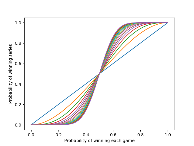
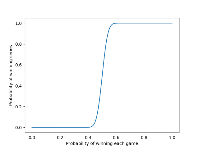
Claiming that you’ve found the maximum value of some function amounts to saying a certain problem has no solution, namely the problem of finding where the function takes on a larger value than the one you claim is optimal. How can you convince a skeptic that you’ve really found the maximum?

You could say “I’ve tried really hard. Here’s a list of things I’ve tried, and see, none of them give a larger value.” Sometimes that’s all you can do. But for convex optimization problems, you can produce a certificate that a skeptic could evaluate that proves that your solution is optimal. More on that here.

Systems of polynomial equations

Now suppose you have a system of polynomial equations. If you’re able to find a solution, then this solution is its own certificate. Want to prove that supposed solution actually is a solution? Plug it in and see.

But how do you prove that you haven’t overlooked any possibilities and there simply isn’t a solution to be found? Once again there is a kind of certificate.

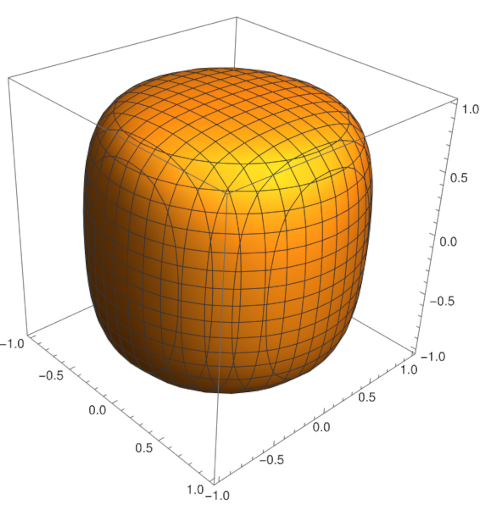
Suppose you have a system of m polynomial equations in n complex variables.

\begin{align*} f_1(z_1, z_2, z_3, \ldots, z_n) &= 0 \\ f_2(z_1, z_2, z_3, \ldots, z_n) &= 0 \\ f_3(z_1, z_2, z_3, \ldots, z_n) &= 0 \\ &\cdots \\ f_m(z_1, z_2, z_3, \ldots, z_n) &= 0 \\ \end{align*}

The system of equations has a solution if and only if the algebraic variety generated by the f‘s is non-empty.

If we can find a polynomial combination of the f‘s that equals 1, i.e. we can find g1 through gm such that

g_1 f_1 + g_2 f_2 + g_3 f_3 + \cdots + g_mf_m = 1

then the variety generated by the f‘s is empty. Such a polynomial combination would be a certificate that the system of equations has no common solution, a certificate of infeasibility. There is an algorithm for finding this polynomial combination, the extended Buchberger algorithm, an analog of the extended Euclidean algorithm.

There is a corresponding theorem for polynomials of a real variable, the so-called positivstellensatz, but it is a little more complicated. The name “complex numbers” is unfortunate because passing to “complex” numbers often simplifies problems.

Related posts

Time difference

A simple question sent me down a rabbit hole this morning: what is the time difference between Houston and London?

At the moment the difference is six hours. But how will that change when Daylight Saving Time ends this year. Wait a minute, will Daylight Saving Time end this year?

I wasn’t even sure whether we were on DST until I asked my wife a few days ago. “Spring forward, Fall back. It’s been Fall for a month now. Did we fall back?”

The US Senate passed the “Sunshine Protection Act” last year that would have eliminated changing times (Yay!) by permanently staying on DST (Boo!). Whatever happened to that? Are we about to fall back or not?

Turns out the House of Representatives never passed the bill, so  things will stay as they have been. Apparently the Senate didn’t seriously consider the Sunshine Protection Act. According to Wikipedia,

In 2022, the Senate passed the bill by unanimous consent, although several senators stated later that they would have objected if they had known that the bill could pass.

OK, so when does the time change in the US? It’s always a Sunday, but which one? Again according to Wikipedia,

Since 2007, in areas of Canada and the United States in which it is used, daylight saving time begins on the second Sunday of March and ends on the first Sunday of November.

Alright, now what about London? Europe has “Summer Time,” which is the same idea as Daylight Saving Time. Summer Time ends on the last Sunday in October.

At the moment, London is 6 hours ahead of Houston. This Sunday, October 29, London falls back an hour and the difference with Houston will be 5 hours. Then the following week it goes back to 6 hours.

In the process of looking into this, I found out that between 1941 and 1945, and again 1947, there was something call British Double Summer Time in which clocks sprung ahead two hours.

Time zones are surprisingly complicated, though mostly for good reasons. I would not recommend abolishing time zones (except for anything done on a computer, in which using UTC internally is the only way to go). But Daylight Saving Time / Summer Time is ridiculous. It made more sense years ago than it does now. Now there is more variety in individual work schedules, and there is more need to coordinate with people outside your time zone.

Best of N series

A couple days ago I wrote about the likelihood of the better team winning a best-of-five or best-of-seven series. That is, if the probability of X winning a game against Y is p > ½, how likely is it that X will win a majority of 5 games or a majority of 7 games.

This assumes the probability of winning each game is fixed and that each game is independent. Actual sports series are more complicated than that.

I was thinking about the baseball playoffs, and so I chose series of 5 and 7. But some tennis fans asked me to add series of 3. And others asked me to add series of more than 7.

As reported in the earlier post,the probability of X winning a series of N games is

\sum_{n > N-n} \binom{N}{n} p^n q^{N-n}

Here is a plot for series of 1, 3, 5, …, 29 games.

Best of N series

The blue diagonal line is the probability of winning each game, i.e. winning a 1-game series.

As you play longer series, the probability of the better team winning increases. Notice that you get the most lift from the diagonal line when playing a 3-game series, the orange line above. You get more lift going from 3 games to 5 games, from the orange line to the green line, though not as much. And as observed in the earlier post, you don’t get much improvement going from 5 games to 7 games, going from green to red.

Even with a series of 29 games, there’s a decent chance that the better team may not win the series, unless the better team is much better. The race is not always to the swift, nor the battle to the strong.

As you keep increasing the number of games N, the slope of the line in the middle becomes steeper, but slowly. You hit diminishing return immediately, with each additional pair of games making less and less difference. Still, the curve is getting steeper. Here’s the curve for a series of 499 games.

Best of 499 games

The slope of the curve in the middle is increasing in proportion to the square root of the number of games.

Related posts

Photo by J. Schiemann on Unsplash

Lessons from Skylab

Skylab 4

I discovered the Space Rocket History Podcast a while back and listened to all the episodes on the Apollo program. I’m now listening to the episodes on Skylab as they come out. I came for Apollo; I stayed for Skylab. I would not have sought out the episodes on Skylab, and that would have been a shame.

Skylab is an underrated program. I wonder how many in my children’s generation even know what Skylab was. Those who do probably think of it as brief interlude between Apollo and the Space Shuttles, or more cynically, a way to keep aerospace contractors in business after the Apollo program ended. But NASA learned a lot during the Skylab program.

The numbering of the Skylab missions is a little confusing. Skylab 1 was the mission to put the lab itself into orbit. The first manned mission to the lab was Skylab 2, the second manned mission was Skylab 3, and the final manned mission was Skylab 4.

Skylab 2 was the most dramatic Skylab mission, just as Apollo 13 was the most dramatic Apollo mission, because in both cases there were major problems to be solved. The missions were literally dramatic in that they had the story arc of a drama.

Because Skylab 2 was primarily concerned with repairs, Skylab 3 was the first mission entirely focused on planned mission objectives. The productivity of the crew started slow and steadily accelerated over the course of the mission. I recommend the Space Rocket History Podcast for the details.

NASA initially scheduled the crew of Skylab 4 to work at the pace Skylab 3 achieved by the end of that mission. This lead to tension, mistakes, and falling behind schedule. Ground control and the astronauts worked through their mutual frustrations and came up with better ways of working together. The crew then exceeded the ground crew’s initial expectations. One change was to distinguish synchronous and asynchronous tasks, letting the crew decide when to do tasks that did not have to be done at a particular point in orbit. Another change was to allow the crew more rest: the crew accomplished more by working less (and making fewer mistakes).

This would make a good business school case study. In fact there was a Harvard Business School case study about Skylab 4, but it was based on false information and presumably drew the wrong lessons from the mission. The case study said the crew went on strike for a day, rebelling against ground control. The truth was that ground control lost radio contact with Skylab for one orbit, 90 minutes, due to an error.

Related posts

Curvature: principal, Gauss, and mean

This post will compute the center of curvature for an object described in the previous post. In order to do that we first need to describe principle curvature and Gauss curvature, and we’ll throw in mean curvature while we’re at it.

Let S be a surface sitting in three dimensional space. No need for more generality to get where we want to go. At any point p on S we can draw curves on the S through p and compute the curvature at p. The curvature is the reciprocal of the radius of the kissing circle.

If we draw curves through p in every direction, some may have larger or smaller curvature than others. Let k1 and k2 be the minimum and maximum curvatures at p. These re the principal curvatures. The product k1 k2 of the principle curvatures is the Gaussian curvature and their average ( k1 + k2)/2 is the mean curvature. Incidentally, when principle curvatures are not equal. the directions in which the curvature is minimized and maximized are orthogonal.

In the previous post I said that the center of curvature for the surface with equation

x^2 + y^2 + (z/h)^2 = s^2 (x^2 + y^2) (z/h)^2 + 1

is finite because the curvature is always positive. In particular, we wanted to know the center of curvature at the bottom, where x = y = 0 and z = −h.

The calculation to get there is messy, but the end result is simple: the principle curvatures are equal by symmetry, and both equal 1 − s². Therefore the center of curvature is at z = 1/(1 − s²).

Calculation details

The following Mathematica code calculates the (signed) curvature of a curve of the form F(x, y) = 0.

k[f_, x_, y_] := (D[f[x, y], y]^2 D[f[x, y], {x, 2}] - 
    2 D[f[x, y], x] D[f[x, y], y] D[f[x, y], {x, 1}, {y, 1}] + 
    D[f[x, y], x]^2 D[f[x, y], {y, 2}]) / (D[f[x, y], x]^2 + 
     D[f[x, y], y]^2)^(3/2)

Define

g[x_, y_] := x^2 + y^2 - s^2 x^2 y^1 - 1

and replace y with z/h. When we evaluate the curvature at x = 0 and simplify

Simplify[k[g, x, y] /. { y -> z/h, x -> 0}, Assumptions -> {h > 0}]

we get

(hs² z) / |z|.

When z = −h we find that the unsigned curvature is 1 − s². In the previous post we assumed h > 1, but the calculation above shows that if h < 1 it’s possible for the curvature to be 0. (Recall s must be between 0 and 1.)

Related posts

An algebraic superegg

One year ago I wrote about a variant of the squircle that is quantitatively close to the customary definition but that has nicer algebraic properties.

That post used the term p-squircle for the usual squircle with equation

|x|^p + |y|^p = 1

where p > 2, and the term s-squircle for the variation with equation

x^2 + y^2 = s^2 x^2 y^2 + 1

where s is between 0 and 1. When p = 2 or s = 0 we get a circle. As p goes to infinity or s = 1 we get a square.

Now the superegg is formed by rotating a squircle about an axis. To match the orientation in the posts I’ve written about supereggs, replace y with z above and rotate about the z-axis. We will also introduce a scaling factor h, dividing z by h.

The superegg analog of the s-squircle would have equation

x^2 + y^2 + (z/h)^2 = s^2 (x^2 + y^2) (z/h)^2 + 1

The s-superegg is much easier to work with (for some tasks) than the p-superegg with equation

\left(\sqrt{x^2 + y^2}\right)^p + |z/h|^p = 1

because the former is a polynomial equation and the latter is transcendental (unless p is an even integer). The s-superegg is an algebraic variety while the p-superegg is not in general.

Here’s a plot with s = 0.9 and h = 1.

This plot was made with the following Mathematica code.

    ContourPlot3D[
        x^2 + y^2 + z^2 == 0.9^2 (x^2 + y^2) z^2 + 1, 
        {x, -1, 1}, {y, -1, 1}, {z, -1, 1}]

Yesterday I said that the p-superegg is stable for all p > 2 because the curvature at the bottom is 0. This means the center of curvature is at infinity, which is above the center of mass.

The s-superegg has positive curvature at the bottom for all 0 < s < 1 and so the center of curvature is finite. As s increases, the superegg becomes more like a cylinder and the center of curvature increases without bound. So the s-superegg will be stable for sufficiently large s.

I calculate the center of curvature in the next post.

Related posts

Nonlinear algebra

What is nonlinear algebra?

Negations are tricky. They may be the largest source of bugs in database queries. You have to carefully think about what exactly are you negating.

Any time you see “non-” attached to something, you have to ask what the context is in which the negation takes place. For example, if you hear someone say “non polar bear,” do they mean a non-polar bear, i.e. any bear besides a polar bear, such as a grizzly bear? Or do they mean non-polarbear, i.e. anything that isn’t a polarbear, such as a giraffe or an espresso machine?

Another subtlety is whether “non” means “definitely not” or “not necessarily.” I specialized in nonlinear PDEs in grad school, and “nonlinear” always meant “not necessarily linear.” I don’t recall ever seeing a theorem that required an operator to not be linear, only theorems that did not require operators to necessarily be linear.

With that introduction, what could nonlinear algebra mean? To many people, it would mean working with equations that contain nonlinear terms, such as solving sin(x) = 2x. The sine function is certainly nonlinear, but it’s not the kind of function algebraists are usually interested in.

To a large extent, the algebraist’s universe consists of polynomials. In that context, “nonlinear” means “polynomials that are not necessarily linear.” So things that are nonlinear in the sense that x³ is nonlinear, not in the sense that sin(x) is nonlinear.

If you think of linear algebra as the math surrounding the solution of systems of linear equations, nonlinear algebra is the math surrounding the solution of systems of polynomial equations. Note that this uses “non” in the “not necessarily” sense: polynomials that are not necessarily linear. Linearity is not assumed, but it’s not excluded either.

You might be thinking “isn’t that just algebraic geometry?” if you’re familiar with algebraic geometry. Strictly speaking the answer is yes, but there’s a difference in connotation if not denotation.

Nonlinear algebra, at least how the term has been used recently, means the application-motivated study of ways to solve polynomial equations. As a recent book review puts it,

Nonlinear algebra’s focus is on computation and applications, and the theoretical results that need to be developed accordingly. Michalek and Sturmfels explain that this name is not just a rebranding of algebraic geometry but that it is intended to capture this focus, and to be more friendly to applied mathematicians, questioning the historic boundaries between pure and applied mathematics.

I like the term nonlinear algebra. Algebraic geometry is a vast subject, and there needs to be a term that distinguishes solving polynomial equations for applications from studying some of the most esoteric math out there. One could argue that the latter is ultimately the proper theory of the former, but a lot of people don’t have the time or abstraction tolerance for that.

The term nonlinear algebra may be better than applied algebraic geometry because the latter could imply that the goal is to master the entire edifice of algebraic geometry and look for applications. Nonlinear algebra implies it is for someone looking to learn math as immediately useful for solving nonlinear equations as linear algebra is for solving linear equations.

Related posts

Stability of a superegg

Three weeks ago I wrote about supereggs, a shape popularized by Piet Hein.

Brass superegg by Piet Hein

One aspect of supereggs that I did not address is their stability. Looking at the photo above, you could imagine that if you gave the object a slight nudge it would not fall over. Your intuition would be right: supereggs are stable.

More interesting than asking whether supereggs are stable is to aks how stable they are. An object is stable if for some ε > 0, a perturbation of size less than ε will not cause the object to fall over.

All supereggs are stable, but the degree of stability decreases as the ratio of height to width increases: the taller the superegg, the easier it is to knock over.

How can we quantify stability? An object is stable if its center of curvature, measured at the point of contact with a horizontal surface, is above its center of mass.

For a sphere, the center of curvature is exactly the center of mass. If we modify the sphere to make it slightly flatter at the point of contact, the center of curvature will move above the center of mass and the modified sphere will be stable. On the other hand, if we made the sphere slightly more curved at the point of contact, the center of curvature would move below the center of mass and the object would be unstable.

The center of curvature is the center of the sphere that best approximates a surface at a point. If our object is a sphere, the hypothetical sphere defining the curvature is the object itself. For an object flatter on bottom than a sphere, the sphere defining center of curvature is larger than the object. The flatter the object, the larger the approximating sphere.

The superegg has zero curvature at the bottom, and so its center of curvature is at infinity. But if you push the superegg slightly, the part touching the horizontal surface is no longer the exact center, the curvature is slightly positive, and so the radius of curvature is finite. The center of mass also moves up slightly as the superegg rocks to the side.

So the center of curvature moves down and the center of mass moves up. At what point do they cross and the object becomes unstable?

Solution outline

The equation of the surface of the superegg is

\left(\sqrt{x^2 + y^2}\right)^p + |z/h|^p = 1

where p > 2 (a common choice is p = 5/2) and h > 1 (a common choice is h = 4/3).

If we tilt the superegg so that its axis of symmetry now makes a small angle θ with the z-axis, we have to answer several questions.

  1. Where does the center of mass go?
  2. What is the new point of contact with the horizontal surface?
  3. Where is the center of curvature?
  4. Is the center of curvature above or below the center of mass?

It’s easier to imagine lifting the superegg up from the surface, rotating it in the air, then lowering it to the surface. That way you don’t have to describe how the superegg rocks.

The superegg is radially symmetric about the vertical axis, so without loss of generality you can imagine the problem is limited to the xz plane.

It’s messy to work out the details, but in principle you could work out how much the superegg can be perturbed and return to its original position. You know a priori that the result will be a decreasing function of h and p.

Related posts

[1] Photo by Malene Thyssen, licensed under the Creative Commons Attribution-Share Alike 3.0 Unported license.

Best-of-five versus Best-of-seven

Suppose that when Team X and Team Y play, the probability that X will win a single game is p and the probability that Y will win is q = 1 − p.

What is the probability that X will win the majority of a series of N games for some odd number N?

We know intuitively that the team more likely to win each game is more likely to win the series. But how much more likely?

We also know intuitively that the more games in the series, the more likely the better team will win. But how much more likely?

The probability of X winning a series of N games is

\sum_{n > N-n} \binom{N}{n} p^n q^{N-n}

It doesn’t matter that maybe not all games are played: some games may not be played precisely because it makes no difference whether they are played. For example, if one team wins the first three in a best-of-five series, the last two games are not played, but for our purposes we may imagine that they were played.

Let’s plot the probability of X winning a best-of-five series and a best-of-seven series.

The better team is more likely to win a series than a game. The probability of the better team winning a single game would be a diagonal line running from (0, 0) to (1, 1). The curves for a series are below this line to the left of 0.5 and above this line to the right of 0.5. But the difference between a best-of-five and a best-of-seven series is small.

Here’s another plot looking at the difference in probabilities, probability of winning best-of-seven minus probability of winning best-of-five.

The maximum difference is between 3% and 4%.

This assumes the probability of winning a game is constant and that games are independent. This is not exactly the case in, for example, the World Series in which human factors make things more complicated.

Related posts

The 19th rule of HIPAA Safe Harbor

The HIPAA Safe Harbor provision says that data can be considered deidentified if 18 kinds of data are removed or reported at low resolution. At the end of the list of 18 items, there is an extra category, sometimes informally called the 19th rule:

The covered entity does not have actual knowledge that the information could be used alone or in combination with other information to identify an individual who is a subject of the information.

So if you otherwise meet the letter of the Safe Harbor provision, but you know (or should know) that the data can still be used to identify people represented in the data, then Safe Harbor does not apply.

The Department of Health and Human Services guidance document gives four examples of “when a covered entity would fail to meet the ‘actual knowledge’ provision.” The first concerns a medical record that would reveal someone’s identity by revealing their profession.

Revealing that someone is a plumber would probably not be a privacy risk, but in the HHS example someone’s occupation was listed as a former state university president. If you know what state this person is in, that greatly narrows down the list possibilities. One more detail, such as age, might be enough to uniquely identify this person.

Free text fields, such as physician notes, could easily contain this kind of information. Software that removes obvious names won’t catch this kind of privacy leak.

Not only are intentional free text fields a problem, so are unintentional free text fields. For example, a database field labeled CASENOTES is probably intended to contain free text. But other text fields, particularly if they are wider than necessary to contain the anticipated data, could contain identifiable information.

If you have data that does not fall under the Safe Harbor provision, or if you are not sure the Safe Harbor rules are enough to insure that the data are actually deidentified, let’s talk.

Related posts

This post is not legal advice. My clients are often lawyers, but I am not a lawyer.