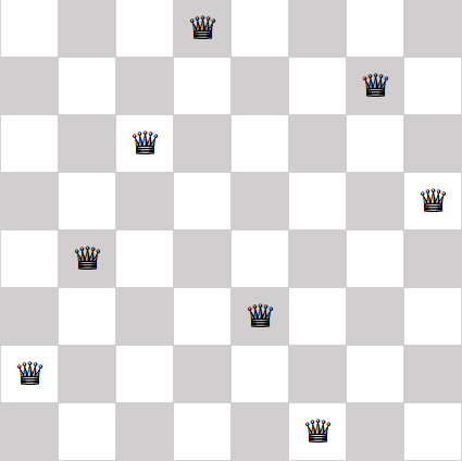
The famous n queens problem is to find a way to position n queens on a n×n chessboard so that no queen attacks any other. That is, no two queens can be in the same row, the same column, or on the same diagonal. Here’s an example solution:
Costas arrays
In this post we’re going to look at a similar problem, weakening one requirement and adding another. First we’re going to remove the requirement that no two pieces can be on the same diagonal. This turns the n queens problem into the n rooks problem because rooks cannot move diagonally.
Next, imagine running stiff wires from every rook to every other rook. We will require that no two wires have the same length and run in the same direction. in more mathematical terms, we require that the displacement vectors between all the rooks are unique.
A solution to this problem is called a Costas array. In 1965, J. P. Costas invented what are now called Costas arrays to solve a problem in radar signal processing.
Why do we call a solution a Costas array rather than a Costas matrix? Because a matrix solution can be described by recording for each column the row number of the occupied cell. For example, we could describe the eight queens solution above as
(2, 4, 6, 8, 3, 1, 7, 5).
Here I’m numbering rows from the bottom up, like points in the first quadrant, rather than top to bottom as one does with matrices.
Note that the solution to the eight queens problem above is not a Costas array because some of the displacement vectors between queens are the same. For example, if we number queens from left to right, the displacement vectors between the first and second queens is the same as the displacement vector between the second and third queens.
Visualizing a Costas array
Here’s a visualization of a Costas array of order 5.
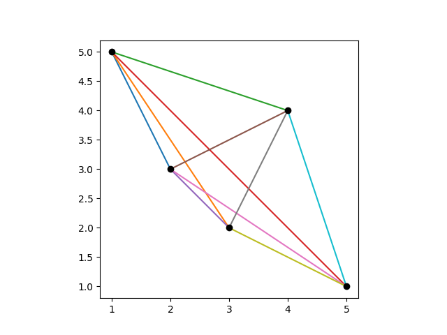
It’s clear from the plot that no two dots are in the same row or column, but it’s not obvious that all the connecting lines are different. To see that the lines are different, we move all the tails of the connecting lines to the origin, keeping their length and direction the same.
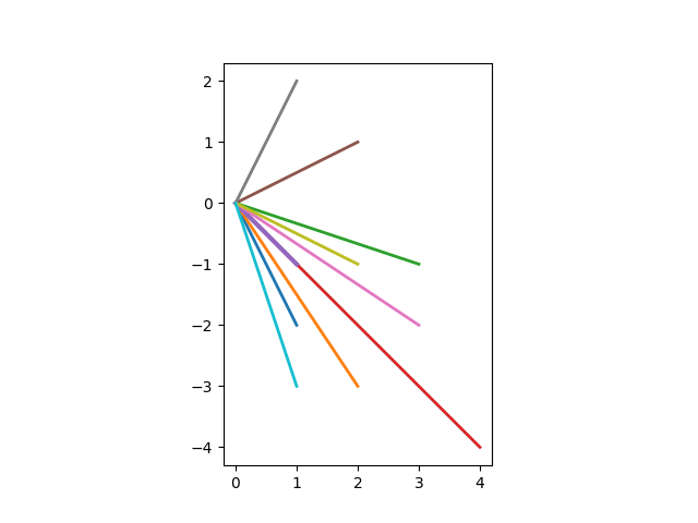
There are 10 colored lines in the first plot, but at first you may only see 9 in the second plot. That’s because two of the lines have the same direction but different length. If you look closely, you’ll see that there’s a short purple line on top of the long red line. That is, one line runs from the origin to (1, -1) and another from the origin to (4, -4).
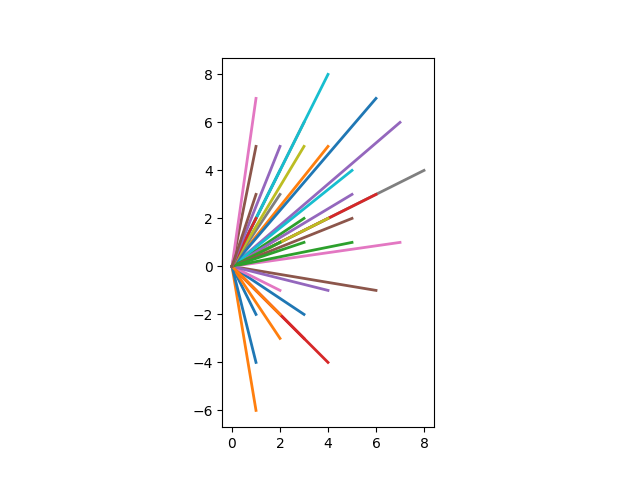
Here is a visualization of a Costas array of order 9.
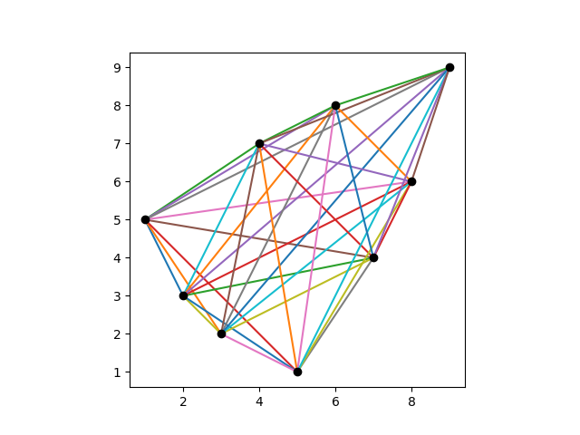
And here are its displacement vectors translated to the origin.
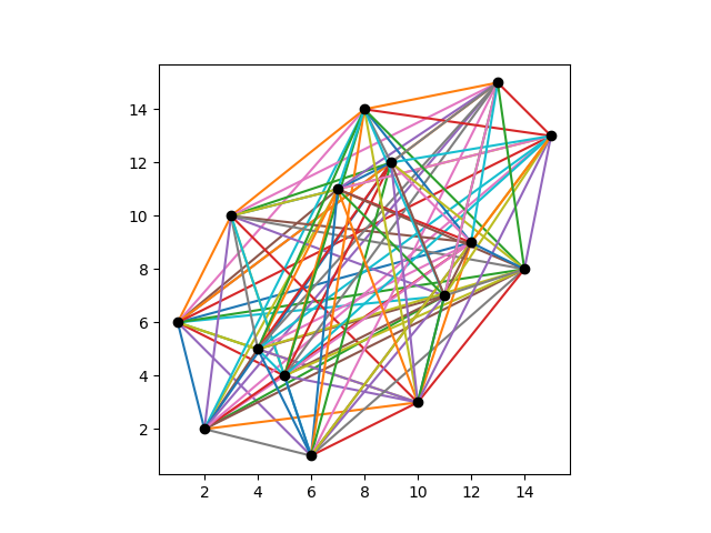
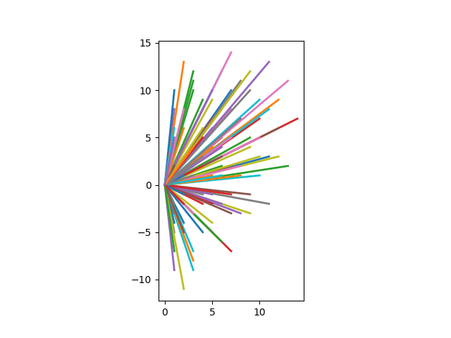
Here is a visualization of a Costas array of order 15.
And here are its displacement vectors translated to the origin.
Generating Costas arrays
There are algorithms for generating some Costas arrays, but not all. Every known algorithm [1] leaves out some solutions, and it is not know whether Costas arrays exist for some values of n.
The Costas arrays above were generated using the Lempel construction algorithm. Given a prime p [2] and a primitive root mod p [3], the following Python code will generate a Costas array of order p – 2.
    p = 11 # prime
    a = 2 # primitive element

    # verify a is a primitive element mod p
    s = {a**i % p for i in range(p)}
    assert( len(s) == p-1 )

    n = p-2
    dots = []

    for i in range(1, n+1):
        for j in range(1, n+1):
            if (pow(a, i, p) + pow(a, j, p)) % p == 1:
                dots.append((i,j))
                break
Related posts
[1] Strictly speaking, no scalable algorithm will enumerate all Costas arrays. You could enumerate all permutation matrices of order n and test whether each is a Costas array, but this requires generating and testing n! matrices and so is completely impractical for moderately large n.
[2] More generally, the Lempel algorithm can generate a solution of order q-2 where q is a prime power. The code above only works for primes, not prime powers. For prime powers, you have to work with finite fields of order q and the code would be more complicated.
[3] A primitive root for a finite field of order q is a generator of the multiplicative group of the field, i.e. an element x such that every non-zero element of the field is some power of x.


