I had heard of the Svalbard Global Seed Vault, but I hadn’t heard of the nearby Arctic World Archive until today. The latter contains source code preserved on film, a format that should last at least 500 years.
Series for π
Here’s a curious series for π that I ran across on Math Overflow.

In case you’re unfamiliar with the notation, n!! is n double factorial, the product of the positive integers up to n with the same parity as n. More on that here.
When n is 0 or -1, n!! is defined to be 1, which is needed above. You could justify this by saying the product is empty, and an empty product is 1. More on that here.
Someone commented on Math Overflow that Mathematica could calculate this sum, so I gave it a try.
    f[j_] := (2 j - 3)!! (2 j - 1)!! /((2 j - 2)!! (2 j + 2)!!)
    Sum[f[j], {j, 1, Infinity}]
Sure enough, Mathematica returns 2/3π.
It’s a slowly converging series as Mathematica can also show.
    In:  N[Sum[f[j], {j, 1, 100}]]
    Out: 0.210629
    In:  N[2/(3 Pi)]
    Out: 0.212207
If you’re curious about series for calculating π that converge quickly, here’s an algorithm that was once used for a world record calculation of π.
Related posts
Morse code numbers and abbreviations
Numbers in Morse code seem a little strange. Here they are:
    |-------+-------|
    | Digit | Code  |
    |-------+-------|
    |     1 | .---- |
    |     2 | ..--- |
    |     3 | ...-- |
    |     4 | ....- |
    |     5 | ..... |
    |     6 | -.... |
    |     7 | --... |
    |     8 | ---.. |
    |     9 | ----. |
    |     0 | ----- |
    |-------+-------|
They’re fairly regular, but not quite. That’s why a couple years ago I thought it would be an interesting exercise to write terse code to encode and decode digits in Morse code. There’s exploitable regularity, but it’s irregular enough to make the exercise challenging.
Design
As with so many things, this scheme makes more sense than it seems at first. When you ask “Why didn’t they just …” there’s often a non-obvious answer.
The letters largely exhausted the possibilities of up to 4 dots and dashes. Some digits would have to take five symbols, and it makes sense that they would all take 5 symbols. But why the ones above? This scheme uses a lot of dashes, and dashes take three times longer to transmit than dots.
A more efficient scheme would be to use binary notation, with dot for 0’s and dash for 1’s. That way the leading symbol would always be a dot and usually the second would be a dot. That’s when encoding digits 0 through 9. As a bonus you could use the same scheme to encode larger numbers in a single Morse code entity.
The problem with this scheme is that Morse code is intended for humans to decode by ear. A binary scheme would be hard to hear. The scheme actually used is easy to hear because you only change from dot to dash at most once. As Morse code entities get longer, the patterns get simpler. Punctuation marks take six or more dots and dashes, but they have simple patterns that are easy to hear.
Code golf
When I posed my coding exercise as a challenge, the winner was Carlos Luna-Mota with the following Python code.
    S="----.....-----"
    e=lambda x:S[9-x:14-x]
    d=lambda x:9-S.find(x)
Honorable mention goes to Manuel Eberl with the following code. It only does decoding, but is quite clever and short.
d=lambda c:hash(c+'BvS+')%10
It only works in Python 2 because it depends on the specific hashing algorithm used in earlier versions of Python.
Cut numbers
If you’re mixing letters and digits, digits have to be five symbols long. But if you know that characters have to be digits in some context, this opens up the possibility of shorter encodings.
The most common abbreviations are T for 0 and N for 9. For example, a signal report is always three digits, and someone may send 5NN rather than 599 because in that context it’s clear that the N’s represent 9s.
When T abbreviates 0 it might be a “long dash,” slightly longer than a dash meant to represent a T. This is not strictly according to Hoyle but sometimes done.
There are more abbreviations, so called cut numbers, though these are much less common and therefore less likely to be understood.
    |-------+-------+-----+--------+----|
    | Digit | Code  |  T1 | Abbrev | T2 |
    |-------+-------+-----+--------+----|
    |     1 | .---- |  17 | .-     |  5 |
    |     2 | ..--- |  15 | ..-    |  7 |
    |     3 | ...-- |  13 | ...-   |  9 |
    |     4 | ....- |  11 | ....-  | 11 |
    |     5 | ..... |   9 | .      |  1 |
    |     6 | -.... |  11 | -....  | 11 |
    |     7 | --... |  13 | -...   |  9 |
    |     8 | ---.. |  15 | -..    |  7 |
    |     9 | ----. |  17 | -.     |  5 |
    |     0 | ----- |  19 | -      |  3 |
    |-------+-------+-----+--------+----|
    | Total |       | 140 |        | 68 |
    |-------+-------+-----+--------+----|
The space between dots and dashes is equal to one dot, and the length of a dash is the length of three dots. So the time required to send a sequence of dots and dashes equals
2(# dots) + 4(# dashes) – 1
In the table above, T1 is the time to transmit a digit, in units of dots, without abbreviation, and T2 is the time with abbreviation. Both the maximum time and the average time are cut approximately in half. Of course that’s ideal transmission efficiency, not psychological efficiency. If the abbreviations are not understood on the receiving end and the receiver asks for numbers to be repeated, the shortcut turns into a longcut.
Related posts
Multiple Frequency Shift Keying
A few days ago I wrote about Frequency Shift Keying (FSK), a way to encode digital data in an analog signal using two frequencies. The extension to multiple frequencies is called, unsurprisingly, Multiple Frequency Shift Keying (MFSK). What is surprising is how MFSK sounds.
When I first heard MFSK I immediately recognized it as an old science fiction sound effect. I believe it was used in the original Star Trek series and other shows. The sound is in once sense very unusual, which is why it was chosen as a sound effect. But in another sense it’s familiar, precisely because it has been used as a sound effect.
Each FSK pulse has two possible states and so carries one bit of information. Each MFSK pulse has 2n possible states and so carries n bits of information. In practice n is often 3, 4, or 5.
Why does it sound strange?
An MFSK signal will jump between the possible frequencies in no apparent; if the data is compressed before encoding, the sequence of frequencies will sound random. But random notes on a piano don’t sound like science fiction sound effects. The frequencies account for most of the strangeness.
MFSK divides its allowed bandwidth into uniform frequency intervals. For example, a 500 Hz bandwidth might be divided into 32 frequencies, each 500/32 Hz apart. The tones sound strange because they are uniformly on a linear scale, whereas we’re used to hearing notes uniformly spaced on a logarithmic scale. (More on that here.)
In a standard 12-note chromatic scale, the ratios between consecutive frequencies is constant, each frequency being about 6% larger than the previous one. More precisely, the ratio between consecutive frequencies equals the 12th root of 2. So if you take the logarithm in base 2, the distance between each of the notes is 1/12.
In MFSK the difference between consecutive frequencies is constant, not the ratio. This means the higher frequencies will sound closer together because their ratios are closer together.
Pulse shaping
As I discussed in the post on FSK, abrupt frequency changes would cause a signal to use an awful lot of bandwidth. The same is true of MFSK, and as before the solution is to taper the pulses to zero on the ends by multiplying each pulse by a windowing function. The FSK post shows how much bandwidth this saves.
When I created the audio files below, at first I didn’t apply pulse shaping. I knew it was important to signal processing, but I didn’t realize how important it is to the sound: you can hear the difference, especially when two consecutive frequencies are the same.
Audio files
The following files are a 5-bit encoding. They encode random numbers k from 0 to 31 as frequencies of 1000 + 1000k/32 Hz.
Here’s what a random sample sounds like at 32 baud (32 frequency changes per second) with pulse shaping.
Here’s the same data a little slower, at 16 baud.
And here is is even slower, at 8 baud.
Examples
If you know of examples of MFSK used as a sound effect, please email me or leave a comment below.
Here’s one example I found: “Sequence 2” from
this page of sound effects sounds like a combination of teletype noise and MFSK. The G7 computer sounds like MFSK too.
Related posts
Dial tone and busy signal
Henry Lowengard left a comment on my post Phone tones in musical notation mentioning dial tones and busy signals, so I looked these up.
Tones
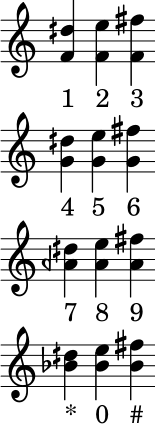
According to this page, a dial tone in DTMF [1] is a chord of two sine waves at 350 Hz and 440 Hz. In musical notation:
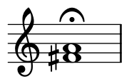
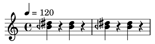
According to the same page, a busy signal is a combination of 480 Hz and 620 Hz with pulses of 1/2 second.
Note that the bottom note is an B half flat, i.e. midway between a B and a B flat, denoted by the backward flat sign. The previous post on DTMF tones also used quarter tone notation because the frequencies don’t align well with a conventional chromatic scale. The frequencies were chosen to be easy to demodulate rather than to be musically in tune.
Audio files
Here are audio files corresponding to the notation above.
Lilypond code for music
Here is the Lilypond code that was used to make the images above.
    \begin{lilypond}
       \new Staff \with { \omit TimeSignature} {
           \relative c'{ 1 \fermata | }
       }
       \new Staff {
            \tempo 4 = 120
            \relative c''{
            <beh dis> r4 <beh dis> r4 | <beh dis> r4 <beh dis> r4 |
            }
        }
    \end{lilypond}
Related posts
[1] Dual-tone multi-frequency signaling, trademarked as Touch-Tone
Solar declination
This post expands on a small part of the post Demystifying the Analemma by M. Tirado.
Apparent solar declination given δ by
δ = sin-1( sin(ε) sin(θ) )
where ε is axial tilt and θ is the angular position of a planet. See Tirado’s post for details. Here I want to unpack a couple things from the post. One is that that declination is approximately
δ = ε sin(θ),
the approximation being particular good for small ε. The other is that the more precise equation approaches a triangular wave as ε approaches a right angle.
Let’s start out with ε = 23.4° because that is the axial tilt of the Earth. The approximation above is a variation on the approximation
sin φ ≈ φ
for small φ when φ is measured in radians. More on that here.
An angle of 23.4° is 0.4084 radians. This is not particularly small, and yet the approximation above works well. The approximation above amounts to approximating sin-1(x) with x, and Taylor’s theorem tells the the error is about x³/6, which for x = sin(ε) is about 0.01. You can’t see the difference between the exact and approximate equations from looking at their graphs; the plot lines lie on top of each other.
Even for a much larger declination of 60° = 1.047 radians, the two curves are fairly close together. The approximation, in blue, slightly overestimates the exact value, in gold.
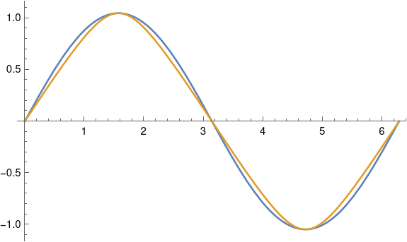
This plot was produced in Mathematica with
    ε = 60 Degree
    Plot[{ε Sin[θ] ], ArcSin[Sin[ε] Sin[θ]]}, {θ, 0, 2π}]
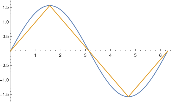
As ε gets larger, the curves start to separate. When ε = 90° the gold curve becomes exactly a triangular wave.
Update: Here’s a plot of the maximum approximation error as a function of ε.

Related posts
Reverse engineering Fourier conventions
The most annoying thing about Fourier analysis is that there are many slightly different definitions of the Fourier transform. One time I got sufficiently annoyed that I creates a sort of Rosetta Stone of Fourier theorems under eight different conventions. Later I discovered that Mathematica supports these same eight definitions, but with slightly different notation.
When I created my Rosetta Stone I wanted to have a set of notes that answered the question “What are the basic Fourier theorems under this convention?” Recently I was reading a reference and wanted to answer the opposite question “Given the theorems this book is stating, what convention must they be using?”
The eight definitions correspond to
![]()
where m is either 1 or 2π, σ is +1 or -1, and q is 2π or 1.
I’m posting these notes for my future reference and for anyone else who may need to do the same sleuthing.
Notation
For the rest of the post, let F and G be the Fourier transforms of f and g respectively. We write
![]()
for the pair of a function and its Fourier transform.
Define the inner product of f and g as
![]()
if f and g are real-value. If the functions are complex-valued, replace g with the complex conjugate if g.
We will sometimes denote the Fourier transform of a function by putting a hat on top of it.
Convolution theorem
The convolution theorem gives a quick way to determine the parameter m. Suppose convolution is defined by
![]()
Then
![]()
and so you can find m immediately. If f*g = F*G with no extra factor out front, m = 1. Otherwise if there’s a factor of √2π out front, then m = 2π. If there’s any other factor, you’ve got an arcane definition of Fourier transform that isn’t one of the eight considered here.
Some authors, like Walter Rudin, include a scaling factor in the definition of convolution, in which casethe argument of this section doesn’t hold.
Parseval and Plancherel
Parseval’s theorem says that the inner product of f and g is proportional to the inner product of F and G. The proportionality constant depends on the definition of Fourier transform, specifically on m and q, and so you can determine m or q from the form of Parseval’s theorem.
![]()
If k = 1, then either q = 2π and m = 1 or q = 1 and m = 2π. If you know m, say from the statement of the convolution theorem, then Parseval’s theorem tells you q.
Plancherel’s theorem is the special case of Parseval’s theorem with f = g. It can be used the same way to solve for m or q.
If k = 2π, then q = m = 1. If k= 1/2π, then q = m = 1.
Double transform
Theorems about taking the Fourier transform twice carry the same information as Parseval’s and Plancherel’s theorems, i.e. they also let you determine m or q.
We have
![]()
with the same conclusions based on k as above:
- If k = 1, then either q = 2π and m = 1 or q = 1 and m = 2π.
- If k = 2π, then q = m = 1.
- If k= 1/2π, then q = m = 1.
Shift and differentiation
So far we none of our theorems have allowed us to reverse engineer σ. Either the shift or differentiation theorem will let is find σq.
The shift theorem says
![]()
where k = σq. Since σ = ±1 and q = 1 or 2π, the product σq determines both σ and q.
Similarly, the differentiation theorem says the Fourier transform of the derivative of f transforms as
![]()
and again k = σq.
Dividing an octave into 14 pieces
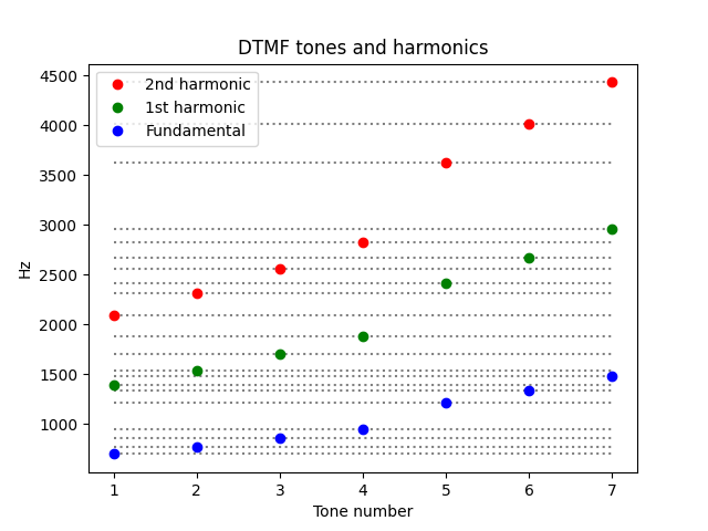
Keenan Pepper left a comment on my previous post saying that the DTMF tones used by touch tone phones “are actually quite close to 14 equal divisions of the octave (rather than the usual 12).”
Let’s show that this is right using a little Python.
    import numpy as np

    freq = np.array([697, 770, 852, 941, 1209, 1336, 1477])
    lg = np.log2(freq)
    spacing = lg[1:] - lg[:-1]
    print(spacing)
    print([2/14, 2/14, 2/14, 5/14, 2/14, 2/14])
If the tones are evenly spaced on a 14-note scale, we’d expect the logarithms base 2 of the notes to differ by multiples of 1/14.
This produces the following:
    [0.144 0.146 0.143 0.362 0.144 0.145]
    [0.143 0.143 0.143 0.357 0.143 0.143]
By dividing the octave into 14 points the DFMT system largely avoids overlap between the set of tones and the set of their harmonics. However, the first overtone of the first tone (1394 Hz) is kinda close to the fundamental of the 6th tone (1336 Hz).
Related posts
Phone tones in musical notation
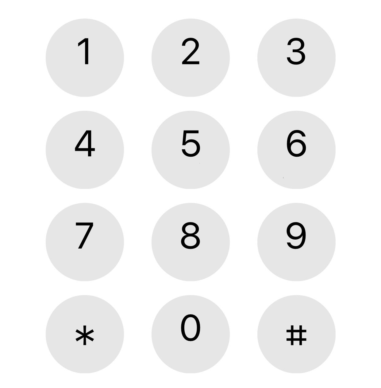
The sounds produced by a telephone keypad are a combination of two tones: one for the column and one for the row. This system is known as DTMF (dual tone multiple frequency).
I’ve long wondered what these tones would be in musical terms and I finally went to the effort to figure it out when I ran across DTMF in [1].
The three column frequencies are 1209, 1336, and 1477 Hz. These do not correspond exactly to standard musical pitches. The first frequency, 1209 Hz, is exactly between a D and a D#, two octaves above middle C. The second frequency, 1336 Hz, is 23 cents [2] higher than an E. The third frequency, 1477 Hz, lands on an F#.
In approximate musical notation, these pitches are two octaves above the ones written below.
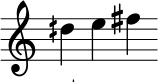
Notice that the symbol in front of the D is a half sharp, one half of the symbol in front of the F.
Similarly, the four row frequencies, starting from the top, are 697, 770, 852, and 941 Hz. In musical terms, these notes are F, G (31 cents flat), A (54 cents flat), and B flat (16 cents sharp).
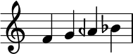
The backward flat symbol in front of the A is a half flat. As with the column frequencies, the row frequencies are two octaves higher than written.
These tones are deliberately not in traditional harmony because harmonic notes (in the musical sense) are harmonically related (in the Fourier analysis sense). The phone company wants tones that are easy to pull apart analytically.
Finally, here are the chords that correspond to each button on the phone keypad.
Update: Dial tone and busy signal
Related posts
[1] Electric Circuits by Nilsson and Riedel, 10th edition, page 548.
[2] A cent is 1/100 of a semitone.
Frequency shift keying (FSK) spectrum
This post will look encoding digital data as an analog signal using frequency shift keying (FSK), first directly and then with windowing. We’ll look at the spectrum of the encoded signal and show that basic FSK uses much less bandwidth than direct encoding, but more bandwidth than FSK with windowing.
Square waves
The most natural way to encode binary data as an analog signal would be represent 0s and 1s by a sequence of pulses that take on the values 0 and 1.
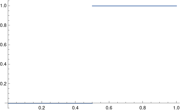
A problem with this approach is that it would require a lot of bandwidth.
In theory a square wave has infinite bandwidth: its Fourier series has an infinite number of non-zero coefficients. In practice, the bandwidth of a signal is determined by how many Fourier coefficients it has above some threshold. The threshold would depend on context, but let’s say we ignore Fourier components with amplitude smaller than 0.001.
As I wrote about here, the nth Fourier sine series coefficients for a square wave is equal to 4/nπ for odd n. This means we would need on the order of 1,000 terms before the coefficients drop below our threshold.
Frequency shift keying
The rate of convergence of the Fourier series for a function f depends on the smoothness of f. Discontinuities, like the jump in a square wave, correspond to slow convergence, i.e. high bandwidth. We can save bandwidth by encoding our data with smoother functions.
So instead of jumping from 0 to 1, we’ll encode a 0 as a signal of one frequency and a 1 as a signal with another frequency. By changing the frequency after some whole number of periods, the resulting function will be continuous, and so will have smaller bandwidth.
Suppose we have a one second signal f(t) that is made of half a second of a 4 Hz signal and half a second of a 6 Hz signal, possibly encoding a 0 followed by a 1.
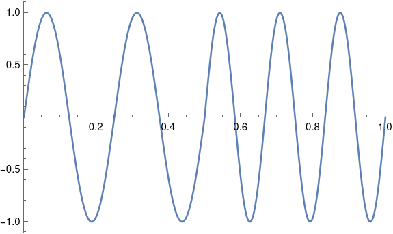
What would the Fourier coefficients look like? If we just had a 4 Hz sine wave, the Fourier series would have only one component: the signal itself at 4 Hz. If we just had a 6 Hz sine wave, the only Fourier component would again be the signal itself. There would be no sine components at other frequencies, and no cosine components.
But our signal patched together by concatenating 4 Hz and 6 Hz signals has non-zero cosine terms for every odd n, and these coefficients decay like O(1/n²).
Our Fourier series is
f(t) = 0.25 sin 8πt + 0.25 sin 12πt + 0.0303 cos 2πt + 0.1112 cos 6πt – 0.3151 cos 12πt + 0.1083 cos 10πt + …
We need to go out to 141 Hz before the coefficients drop below 0.001. That’s a lot of coefficients, but it’s an order of magnitude fewer coefficients than we’d need for a square wave.
Pulse shaping
Although our function f is continuous, it is not differentiable. The left-hand derivative at 1/2 is 8π and the right-hand derivative is 12π. If we could replace f with a related function that is differentiable at 1/2, presumably the signal would require less bandwidth.
We could do this by multiplying both halves of our signal by a windowing function. This is called pulse shaping because instead of a simple sine wave, we change the shape of the wave, tapering it at the ends.
Let’s using a cosine window because that’ll be easy; in practice you’d probably use a different window [1].
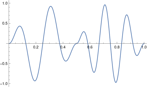
Now our function is differentiable at 1/2, and its Fourier series converges more quickly. Now we can disregard components above 40 Hz. With a smoother windowing function the windowed function would have more derivatives and we could disregard more of the high frequencies.
Related posts
[1] This kind of window is called a cosine window because you multiply your signal by one lobe of a cosine function, with the peak in the middle of the signal. Since we’re doing this over [0. 1/2] and again over [1/2, 1], we’re actually multiplying by |sin 2πt|.