Calculating the period of Van der Pol oscillators

A few days ago I wrote about how to solve differential equations with SciPy’s ivp_solve function using Van der Pol’s equation as the example. Van der Pol’s equation is

{d^2x \over dt^2}-\mu(1-x^2){dx \over dt}+x= 0

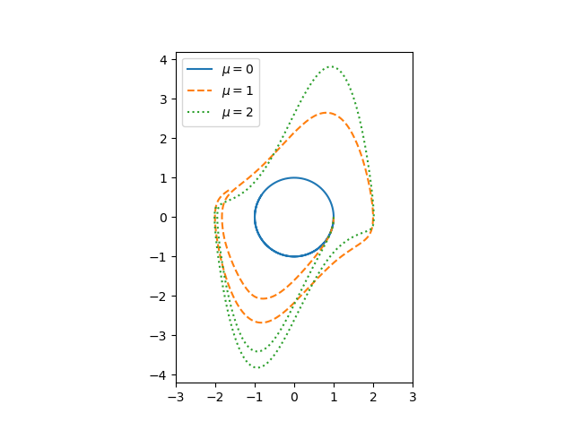
The parameter μ controls the amount of nonlinear damping. For any initial condition, the solution approach a periodic solution. The limiting periodic function does not depend on the initial condition [1] but does depend on μ. Here are the plots for μ  = 0, 1, and 2 from the previous post.

Van der Pol oscillator solutions as a function of time

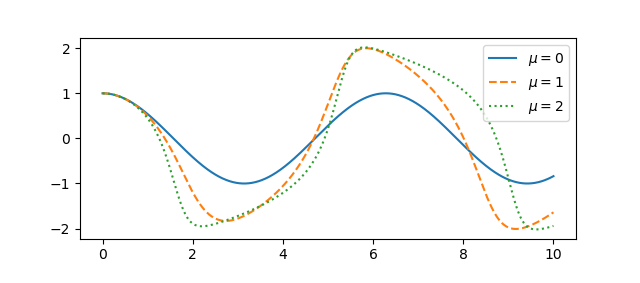
A couple questions come to mind. First, how quickly do the solutions become periodic? Second, how does the period depend on μ? To address these questions, we’ll use an optional argument to ivp_solve we didn’t need in the earlier post.

Using events in ivp_solve

For ivp_solve an event is a function of the time t and the solution y whose roots the solver will report. To determine the period, we’ll look at where the solution is zero; our event function is trivial since we want to find the roots of the solution itself.

Recall from the earlier post that we cast our second order ODE as a pair of first order ODEs, and so our solution is a vector, the function x and its derivative. So to find roots of the solution, we look at what the solver sees as the first component of the solver. So here’s our event function:

    def root(t, y): return y[0]

Let’s set μ = 2 and find the zeros of the solution over the interval [0, 40], starting from the initial condition x(0) = 1, x‘(0) = 0.

    mu = 2
    sol = solve_ivp(vdp, [0, 40], [1, 0], events=root)
    zeros = sol.t_events[0]

Here we reuse the vdp function from the previous post about the Van der Pol oscillator.

To estimate the period of the limit cycle we look at the spacing between zeros, and how that spacing is changing.

    spacing = zeros[1:] - zeros[:-1]
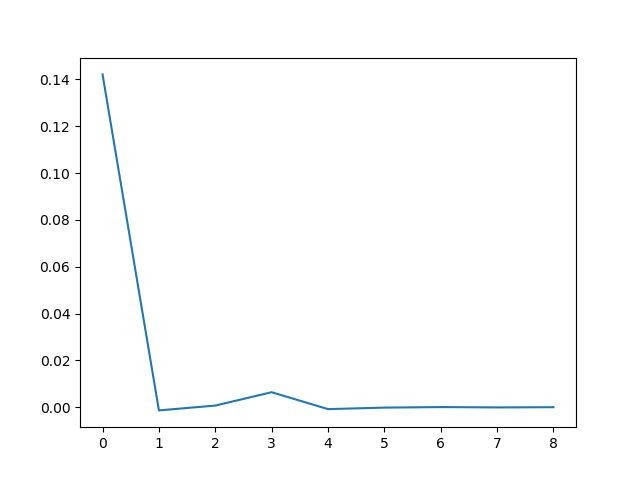
    deltas = spacing[1:] - spacing[:-1]

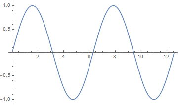
If we plot the deltas we see that the zero spacings quickly approach a constant value. Zero crossings are half periods, so the period of the limit cycle is twice the limiting spacing between zeros.

Van der pol period deltas

Theoretical results

If μ = 0 the Van der Pol oscillator reduces to a simple harmonic oscillator and the period is 2π. As μ increases, the period increases.

For relatively small μ we can calculate the period as above, but as μ increases this becomes more difficult numerically [2]. But one can easily show that the period is asymptotically

T ~ (3 − 2 log 2) μ

as μ goes to infinity. A more refined estimate due to Mary Cartwright is

T ~ (3 − 2 log 2) μ + 2π/μ1/3

for large μ.

More VdP posts

[1] There is a trivial solution, x = 0, corresponding to the initial conditions x(0) = x‘(0) = 0. Otherwise, every set of initial conditions leads to a solution that converges to the periodic attractor.

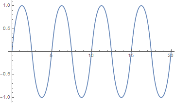
[2] To see why large values of μ are a problem numerically, here’s a plot of a solution for μ = 100.

Solution to Van der Pol for large damping parameter mu

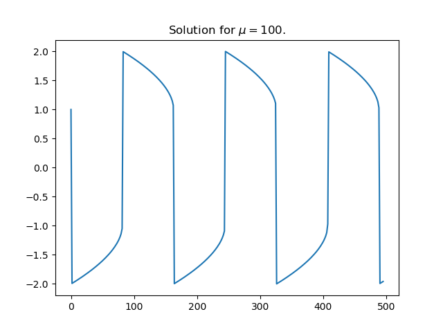
The solution is differentiable everywhere, but the derivative changes so abruptly at the maxima and minima that it is discontinuous for practical purposes.

Solving Van der Pol equation with ivp_solve

Van der Pol’s differential equation is

{d^2x \over dt^2}-\mu(1-x^2){dx \over dt}+x= 0

The equation describes a system with nonlinear damping, the degree of nonlinearity given by μ. If μ = 0 the system is linear and undamped, but as μ increases the strength of the nonlinearity increases. We will plot the phase portrait for the solution to Van der Pol’s equation in Python using SciPy’s new ODE solver ivp_solve.

The function ivp_solve does not solve second-order systems of equations directly. It solves systems of first-order equations, but a second-order differential equation can be recast as a pair of first-order equations by introducing the first derivative as a new variable.

\begin{align*} {dx \over dt} &= y \\ {dy \over dt}&= \mu(1-x^2)y -x \\ \end{align*}

Since y is the derivative of x, the phase portrait is just the plot of (x, y).

Phase portait of Van der Pol oscillator

If μ = 0, we have a simple harmonic oscillator and the phase portrait is simply a circle. For larger values of μ the solutions enter limiting cycles, but the cycles are more complicated than just circles. These limiting cycles are periodic attractors: every non-trivial solution converges to the limit cycle.

Here’s the Python code that made the plot.

from scipy import linspace
from scipy.integrate import solve_ivp
import matplotlib.pyplot as plt

def vdp(t, z):
    x, y = z
    return [y, mu*(1 - x**2)*y - x]

a, b = 0, 10

mus = [0, 1, 2]
styles = ["-", "--", ":"]
t = linspace(a, b, 500)

for mu, style in zip(mus, styles):
    sol = solve_ivp(vdp, [a, b], [1, 0], t_eval=t)
    plt.plot(sol.y[0], sol.y[1], style)
  
# make a little extra horizontal room for legend
plt.xlim([-3,3])    
plt.legend([f"$\mu={m}$" for m in mus])
plt.axes().set_aspect(1)

To plot the solutions as a function of time, rather than plotting phase portraits, change the line

    plt.plot(sol.y[0], sol.y[1], style)

to

    plt.plot(sol.t, sol.y[0], style)

and comment out the line setting xlim This gives the following plot.

Van der Pol oscillator solutions as a function of time

More dynamical system posts

Stability criteria in a nutshell

A continuous linear system is stable if and only if all its eigenvalues have negative real parts.

There are various other stability criteria, but they boil down to the statement above. For example, there is the Routh stability criterion and the Hurwitz stability criterion. There’s also a continued fraction criterion.

But these criteria are just algorithms for determining whether the roots of the characteristic polynomial are all negative; they’re not independent criteria. They were more important in the days of hand calculations; now it’s easy enough to simply compute the roots of the characteristic polynomial numerically.

A discrete-time linear system is stable if and only if all its eigenvalues are inside the unit circle. The change of variables

w = (z − 1) / (z + 1)

maps the interior of the unit disk to the open left half plane, and so the roots of the characteristic polynomial in z are inside the unit circle if and only if the roots of the corresponding function of w are in the left half plane.

Related post: Cayley-Hamilton theorem

Self-curvature

If you look at a sine wave, its curvature is sorta like its values. When sine is zero, the curve is essentially a straight line, and the curvature is zero. When sine is at its maximum, the function bends the most and so the curvature is at a maximum.

This makes sense analytically. The second derivative is something like curvature, and the second derivative of sin(x) is -sin(x). The negative sign suggests that if we look at signed curvature rather than absolute curvature, then the values of a sine curve are roughly proportional to the negative of the curvature at each point.

Here’s a plot showing sin(x) and its negative curvature.

Plot of a sine wave and its curvature

Steven Wilkinson wrote an article [1] addressing the question of whether there is a curve so that the curvature at each point is proportional to the value of the curve. The curvature of a graph of y = y(x) is

\kappa(x) = \frac{y''(x)}{(1 + y'(x)^2)^{3/2}}

and so a curve that is proportional to its curvature is a solution to the nonlinear differential equation

y(x) = \frac{a\, y''(x)}{(1 + y'(x)^2)^{3/2}}

General theory says that there should at least be a solution in a (possibly small) neighborhood of 0, but it’s not obvious a priori that interesting solutions exist. It turns out that if we pick the proportionality constant a = −1 and the initial conditions y(0) = 0 and y ‘(0) = √3 then we get a periodic solution that looks something like a sine.

The following Mathematica code will plot the function for us.

    s = NDSolve[
        {y''[x] = -y[x] (1 + y'[x]^2)^(-3/2), 
        y[0] == 0, y'[0] == Sqrt[3]}, 
         y, {x, 0, 10}]

    Plot[Evaluate[{y[x] /. s}], {x, 0, 10}]

The plot looks a lot like a sine wave. In fact, I imagine that when asked to draw a sine wave, most people would draw something that looks more like this than like an actual sine wave.

Related posts

[1] Steven Wilkison. Self-Curvature Curves. Mathematics Magazine, Vol. 82, No. 5 (December 2009), pp. 354-359

Elementary solutions to differential equations

Differential equations rarely have closed-form solutions. Some do, and these are emphasized in textbooks.

For this post we want to look specifically at homogeneous second order linear equations:

y ” + a(x) y‘ + b(x) y = 0.

If the coefficient functions a and b are constant, then the solution can be written down in terms of elementary functions, i.e. functions a first year calculus student would recognize. This would include, for example, polynomials, sines, and cosines, but would not include, the gamma function, Bessel functions, Airy functions, etc.

If the coefficients a and b are not constant, the differential equation usually does not have an elementary solution. In fact, you might wonder if it is ever possible in that case for the differential equation to have an elementary solution. Experience would suggest not.

A paper by Kovacic [1] thoroughly answers this question. The author gives algorithms for determining whether elementary solutions exist and how to find them if they do exist. The following example comes from that paper.

Consider the equation

y” + ry = 0

where [2]

r(x) = (4 x6 − 8 x5 + 12 x4 + 4 x3 + 7 x2 − 20 x + 4)/4 x4.

Then

y(x) = x−3/2 (x2 − 1) exp(x2/2 − x − 1/x)

is a solution, which the following Mathematica code verifies by evaluating to 0.

r[x_] := (4 x^6 - 8 x^5 + 12 x^4 + 4 x^3 + 7 x^2 - 20 x + 4)/(4 x^4)
f[x_] := x^(-3/2) (x^2 - 1) Exp[x^2/2 - x - 1/x]
Simplify[D[f[x], {x, 2}] - r[x] f[x]]

More differential equation posts

[1] Jerald J. Kovacic. An algorithm for solving second order linear homogeneous differential equations. Journal of Symbolic Computation (1986) 2, 3–43.

[2] There’s an error in the paper, where the denominator of r is given as 4x rather than 4x4.

Numerical methods blog posts

I recently got a review copy of Scientific Computing: A Historical Perspective by Bertil Gustafsson. I thought that thumbing through the book might give me ideas for new topics to blog about. It still may, but mostly it made me think of numerical methods I’ve already blogged about.

In historical order, or at least in the order of Gustafsson’s book:

The links above include numerical methods I have written about. What about the methods I have not written about?

PDEs

I like to write fairly short, self-contained blog posts, and I’ve written about algorithms compatible with that. The methods in Gustafsson’s book that I haven’t written about are mostly methods in partial differential equations. I don’t see how to write short, self-contained posts about numerical methods for PDEs. In any case, my impression is that not many readers would be interested. If you are one of the few readers who would like to see more about PDEs, you may enjoy the following somewhat personal rambling about PDEs.

I studied PDEs in grad school—mostly abstract theory, but also numerical methods—and expected PDEs to be a big part of my career. I’ve done some professional work with differential equations, but the demand for other areas, particularly probability and statistics, has been far greater. In college I had the impression that applied math was practically synonymous with differential equations. I think that was closer to being true a generation or two ago than it is now.

My impression of the market demand for various kinds of math is no doubt colored by my experience. When I was at MD Anderson we had one person in biomathematics working in PDEs, and then none when she left. There may have been people at MDACC doing research into PDEs for modeling cancer, but they weren’t in the biostatistics or biomathematics departments. I know that people are working with differential equations in cancer research, but not at the world’s largest cancer center, and so I expect there aren’t many doing research in that area.

Since leaving MDACC to work as a consultant I’ve seen little demand for differential equations, more in Kalman filters than in differential equations per se. A lot of companies hire people to numerically solve PDEs, but there don’t seem to be many who want to use a consultant for such work. I imagine most companies with an interest in PDEs are large and have a staff of engineers and applied mathematicians working together. There’s more demand for statistical consulting because companies are likely to have an occasional need for statistics. The companies that need PDEs, say for making finite element models of oil reservoirs or airplanes, have an ongoing need and hire accordingly.

Interlaced zeros of ODEs

Sturm’s separation theorem says that the zeros of independent solutions to an equation of the form

y'' + p(x)y' + q(x)y = 0

alternate. That is, between any two consecutive zeros of one solution, there is exactly one zero of the other solution. This is an important theorem because a lot of differential equations of this form come up in applications.

If we let p(x) = 0 and q(x) = 1, then sin(x) and cos(x) are independent solutions and we know that their zeros interlace. The zeros of sin(x) are of the form nπ, and the zeros of cos(x) are multiples of (n + 1/2)π.

What’s less obvious is that if we take two different linear combinations of sine and cosine, as long as they’re not proportional, then their zeros interlace as well. For example, we could take f(x) = 3 sin(x) + 5 cos(x) and g(x) = 7 sin(x) − 11 cos(x). These are also linearly independent solutions to the same differential equation, and so the Sturm separation theorem says their roots have to interlace.

If we take p(x) = 1/x and q(x) = 1 − (ν/x)² then our differential equation becomes Bessel’s equation, and the Bessel functions Jν and Yν are independent solutions. Here’s a little Python code to show how the zeros alternate when ν = 3.

    import matplotlib.pyplot as plt
    from scipy import linspace
    from scipy.special import jn, yn

    x = linspace(4, 30, 100)
    plt.plot(x, jn(3, x), "-")
    plt.plot(x, yn(3, x), "-.")
    plt.legend(["$J_3$", "$Y_3$"])
    plt.axhline(y=0,linewidth=1, color="k")
    plt.show()

Plotting Bessel functions J_3 and Y_3

More differential equation posts

System of Jacobi elliptic functions

Jacobi’s elliptic functions are sorta like trig functions. His functions sn and cn have names that reminiscent of sine and cosine for good reason. These functions come up in applications such as the nonlinear pendulum (i.e. when θ is too
large to assume θ is a good enough approximation to sin θ) and in conformal mapping.

I ran across an article [1] yesterday that shows how Jacobi’s three elliptic functions—sn, cn, and dn—could be defined by one dynamical system

\begin{eqnarray*} x' &=& yz \\ y' &=& -zx \\ z' &=& -k^2 xy \end{eqnarray*}

with initial conditions x(0) = 0, y(0) = 1, and z(0) = 1.

The parameter k is the modulus. (In Mathematica’s notation below, k² is the parameter. See this post on parameterization conventions.) As k decreases to 0, sn converges to sine, cn to cosine, and dn to 1. As k increases to 1, sn converges tanh, and cn and dn converge to sech. So you could think of k as a knob you turn to go from being more like circular functions (ordinary trig functions) to more like hyperbolic functions.

Since we have a dynamical system, let’s plot the solution, varying the modulus each time.The Jacobi functions are periodic (in fact they’re doubly periodic) and so the plots will be closed loops.

f[t_, m_] = {JacobiSN[t, m], JacobiCN[t, m], JacobiDN[t, m]}
ParametricPlot3D[f[t, 0.707], {t, 0, 10}, AspectRatio -> 1]

phase portrait k = 1/2

ParametricPlot3D[f[t, 0.99], {t, 0, 20}, AspectRatio -> 1]

phase portrait k = 1/2

ParametricPlot3D[f[t, 0.01], {t, 0, 20}, AspectRatio -> 1]

phase portrait k = 1/2

Note that this last plot is nearly flat because the modulus is small and so z is nearly constant. The small modulus also makes the phase portrait nearly circular because x is approximately sine and y is approximately cosine.

[1] Kenneth R. Meyer. Jacobi Elliptic Functions from a Dynamical Systems Point of View. The American Mathematical Monthly, Vol. 108, No. 8 (Oct., 2001), pp. 729-737

Duffing equation for nonlinear oscillator

The Duffing equation is an ordinary differential equation describing a nonlinear damped driven oscillator.

\frac{d^2x}{dt} + h\frac{dx}{dt} + \Omega_0^2 x + \mu x^3 = F \cos \omega t

If the parameter μ were zero, this would be a damped driven linear oscillator. It’s the nonlinear x³ term that makes things nonlinear and interesting.

Using an analog computer in 1961, Youshisuke Ueda discovered that this system was chaotic. It was the first discovery of chaos in a second-order non-autonomous periodic system. Lorenz discovered his famous Lorenz attractor around the same time, though his system is third order.

Ueda’s system has been called “Ueda’s strange attractor” or the “Japanese attractor.”

In the linear case, when μ = 0, the phase portrait simply spirals outward from the origin towards its steady state.

But things get much more interesting when μ = 1. Here’s Mathematica code to numerically solve the differential equation and plot the phase portrait.

duff[t_] = 
    NDSolve[{x''[t] + 0.05 x'[t] + x[t] + x[t]^3 == 7.5 Cos[t], 
             x[0] == 0, x'[0] == 1}, x[t], {t, 0, 100}][[1, 1, 2]]
ParametricPlot[{duff[t], duff'[t]}, {t, 0, 50}, AspectRatio -> 1]

Here’s the same system integrated out further, to t = 200 rather 50.

Source: Wanda Szemplińska-Stupnicka. Chaos, Bifurcations and Fractals Around Us.

Asymptotic solution to ODE

Our adventure starts with the following ordinary differential equation:

y' = y = \frac{1}{x}

Analytic solution

We can solve this equation in closed-form, depending on your definition of closed-form, by multiplying by an integrating factor.

e^x y' + e^x y = \frac{e^x}{x}

The left side factors to

(e^x y)'

and so

y = e^{-x} \left( \int^x \frac{e^t}{t}\, dt + c\right)

The indefinite integral above cannot be evaluated in elementary terms, though it can be evaluated in terms of special functions.

We didn’t specify where the integration starts or the constant c. You can make the lower limit of integration whatever you want, and the value of c will be whatever is necessary to satisfy initial conditions.

The initial conditions hardly matter for large x because the constant c is multiplied by a negative exponential. As we’ll see below, the solution y decays like 1/x while the effect of the initial condition decays exponentially.

Asymptotic series solution

I wrote a few months ago about power series solutions for differential equations, but that approach won’t work here, not over a very large range. If y has a Taylor series expansion, so does it’s derivative, and so y‘ + y has a Taylor series. But the right side of our differential equation has a singularity at 0.

What if instead of assuming y has a Taylor series expansion, we assume it has a Laurent series expansion? That is, instead of assuming y is a weighted sum of positive powers of x, we assume it’s a weighted sum of negative powers of x:

y = \sum_{n=1}^\infty a_nx^{-n}

Then formally solving for the coefficients we find that

y = \frac{1}{x} + \frac{1}{x^2} + \frac{2}{x^3} + \cdots + \frac{(n-1)!}{x^n} + \cdots


There’s one problem with this approach: The series diverges for all x because n! grows faster than xn.

And yet the series gives a useful approximation! With a convergent series, we fix x and let n go to infinity. The divergent series above is an asymptotic series, and so we fix n and let x go to infinity.

To see how well the asymptotic solution compares to the analytic solution, we’ll pick the lower limit of integration to be 1 and pick c = 0 in the analytic solution.

The plot above shows the analytic solution, and the first and second order asymptotic solutions. (The nth order solution takes the first n terms of the asymptotic series.) Note that the three curves differ substantially at first but quickly converge together.

Now let’s look at the relative error.

That’s interesting. Eventually the second order approximation is more accurate than the first order, but not at first. In both cases the relative error hits a local minimum, bounces back up, then slowly decreases.

Does this pattern continue if we move on to a third order approximation. Yes, as illustrated below.

Superasymptotic series

The graphs above suggests that higher order approximations are more accurate, eventually, but we might do better than any particular order by letting the order vary, picking the optimal order for each x. That’s the idea behind superasymptotics. For each x, the superasymptotic series sums up terms in the asymptotic series until the terms start getting larger.

When this approach works, it can produce a series that converges exponentially fast, even though each truncated asymptotic series only converges polynomially fast.

Update: To get an idea how accuracy varies jointly with the argument x and the asymptotic approximation order n, consider the following graph. Note that the horizontal axis is now n, not x. The different curves correspond to different values of x, generally moving down as x increases.

Relative error as a function of asymptotic order

Every curve is non-monotone because for every value of x, increasing the order only helps to a point. Then the error gets worse as the series diverges. But as you can see from the graph, you can do quite well by picking the optimal approximation order for a given x.

Related math posts