Triple factorials and Airy functions

Last week I wrote in a post on multifactorials in which I said that

Double factorials come up fairly often, and sometimes triple, quadruple, or higher multifactorials do too.

This post gives a couple examples of triple factorials in practice.

One example I wrote about last week. Triple factorial comes up when evaluating the gamma function at an integer plus 1/3. As shown here,

\Gamma\left(n + \frac{1}{3}\right) = \frac{(3n-2)!!!}{3^n} \Gamma\left(\frac{1}{3}\right)

Another example involves solutions to Airy’s differential equation

y'' - xy = 0

One pair of independent solutions consists of the Airy functions Ai(x) and Bi(x). Another pair consists of the functions

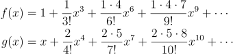
\begin{align*} f(x) &= 1 + \frac{1}{3!}x^3 + \frac{1\cdot 4}{6!}x^6 + \frac{1\cdot 4 \cdot 7}{9!}x^9 + \cdots \\ g(x) &= x + \frac{2}{4!}x^4 + \frac{2\cdot 5}{7!}x^7 + \frac{2\cdot 5 \cdot 8}{10!}x^{10} + \cdots \end{align*}

given in A&S 10.4.3. Because both pairs of functions solve the same linear ODE, each is a linear combination of the other.

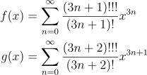
Notice that the numerators are triple factorials, and so the series above can be rewritten as

\begin{align*} f(x) &= \sum_{n=0}^\infty \frac{(3n+1)!!!}{(3n+1)!} x^{3n}\\ g(x) &= \sum_{n=0}^\infty \frac{(3n+2)!!!}{(3n+2)!} x^{3n+1} \end{align*}

The next post gives an example of quadruple factorials in action.

Nonlinear ODEs with stable limit cycles

It’s not obvious when a nonlinear differential equation will have a periodic solution, or asymptotically approach a periodic solution. But there are theorems that give sufficient conditions. This post is about one such theorem.

Consider the equation

x” + f(x) x‘ + g(x) = 0

where f and g are analytic and define F(x) to be the integral of f(t) from 0 to x. The following six hypotheses are sufficient to guarantee that the equation above has a stable limit cycle [1].

  1. g is an odd function,
  2. g is positive for positive x,
  3. f is an even function,
  4. f(o) < 0,
  5. F(x) → ∞ as x → ∞,
  6. F has a unique positive zero.

These hypotheses are satisfied, for example, by Van der Pol’s equation.

Let’s make up coefficient functions f and g that satisfy the conditions above and look for the limit cycle.

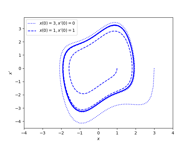
We can let g(x) = x³ and f(x) = x² − 1. And here’s what we get:

The graph shows phase portraits for two different initial conditions, given in the legend of the plot. Note that limit cycle appears solid blue because the trajectories of both the dashed line and the dotted line run around the periodic attractor.

Related posts

[1] You can find this theorem in Topics in Ordinary Differential Equations by William Lakin and David Sanchez.

Linear ODEs with periodic solutions

Suppose we have a differential equation of the form

x” + b(t) x‘ + c(t) x = f(t)

where the functions b and c are periodic with the same period T.

When does the equation above have a solution with period T?

It turns out [1] the equation above will have a T-periodic solution for all T-periodic functions f if and only if the equation

x” + b(t) x‘ + c(t) x = 0

does not have a T-periodic solution. In other words, the non-homogeneous equation has a T-periodic solutions for all f if and only if the homogeneous equation does not [2].

This theorem may not sound right at first. You might think the homogeneous equation having a periodic solution would help if you were looking for a solution to the non-homogeneous equation. An example will show this isn’t the case.

Example

Let’s look at the special case of b = 0, c = a positive constant, and f(t) = cos ωt. As shown here, the natural frequency of the equation is

ω0 = √c

and the homogeneous equation has general solution

x(t) = R cos(ω0t – φ)

for some amplitude R and phase φ.

Also, the non-homogeneous equation has a solution

cos(ωt) /(ω02 – ω2).

So does this contradict the theorem above? Here both the homogeneous and non-homogeneous equations have periodic solutions. However, they don’t have periodic solutions with the same period. The homogeneous solutions have period 2π/ω0, and the non-homogeneous solution has period 2π/ω.

The non-homogeneous solution above requires the driving frequency ω to be different from the natural frequency ω0 or else the denominator would be 0.

If the driving frequency does equal the natural frequency, the non-homogeneous equation does have a solution, but the solution is not periodic. The solutions blows up due to resonance. The non-homogeneous equation has a solution

(t/2ω) sin ωt.

and so the amplitudes of the oscillations grow as t grows. With each period, more energy is pumped into the system and the energy increases without bound.

More general periods

The full set of solutions to a non-homogeneous equation is given by the general solution to the homogeneous equation plus any particular solution to the non-homogeneous equation.

If the driving frequency ω does not equal the natural frequency ω0 then in the example above the homogeneous and non-homogeneous solutions are both periodic, but with different periods. Is their sum periodic? Maybe.

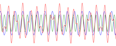
The sum of two periodic functions may or may not be periodic. The image below is from this post where I give an example of two periodic functions, the green and blue lines, whose sum, the red line, is not periodic but rather quasiperiodic.

two periodic functions adding to a quasiperiodic function

The sum of two periodic functions is periodic if the ratio of their periods is a rational number. In the example above, the ratio is the golden ratio, an irrational number.

The general solutions to the non-homogeneous equation above are periodic if and only if the ratio of ω to ω0 is rational.

Contradiction?

But if ω/ω0 is rational, do we have a contradiction to our theorem above? For example, suppose the natural frequency ω0 is 2π and the driving frequency ω is 4π. The the homogeneous solutions have period 1 and the particular solution to the non-homogeneous equation has period 1/2. But a function of period 1/2 also has period 1.

In our case, the equation

x” + 4π² x = 0

has solutions of period 1, and the equation

x” + 4π² x = cos 4πt

also has a solution with period 1.

To see why this isn’t a contradiction, we have to go back and read the theorem more carefully. It says the equation

x” + b(t) x‘ + c(t) x = f(t)

has a T-periodic solution for all T-periodic functions f if and only if the equation

x” + b(t) x‘ + c(t) x = 0

does not have a T-periodic solution.

In our case the homogeneous equation has solutions with period 1, and the non-homogeneous equation also has a solution with period 1. But this is just for one particular forcing function f. The theorem makes a claim for all functions f, and so we have not found a contradiction.

As long as there is some function f(t) with period 1 for which the non-homogeneous equation has no solution with period 1 then the theorem is correct. And in fact we’ve already given an example of such a function, namely cos 2πt. In that case the natural frequency and driving frequency are the same, and the solutions are not periodic due to resonance.

Related posts

[1] See Topics in Ordinary Differential Equations by William Lakin and David Sanchez.

[2] A differential equation in the form above is called homogeneous if the forcing function on the right side is 0 and it is called non-homogeneous if the forcing function is not zero.

[3] If the driving frequency ω does not equal the natural frequency ω0 is the solution periodic even if it doesn’t have the same period

Nonlinear phase portrait

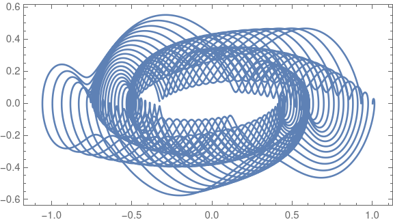
I was reading through Michael Trott’s Mathematica Guidebook for Programming and ran across the following plot.

I find the image aesthetically interesting. I also find it interesting that the image is the phase portrait of a differential equation whose solution doesn’t look that interesting. That is, the plot of (x(t), x ‘(t)) is much more visually interesting than the plot of x(t).

The differential equation whose phase portrait is plotted above is

x''(t) + \frac{1}{20}x'(t)^3 + \frac{1}{5} x(t) = \frac{1}{3}\cos(et)

with initial position 1 and initial velocity 0. It’s a familiar damped, driven harmonic oscillator, except the equation is nonlinear because the derivative term is cubed.

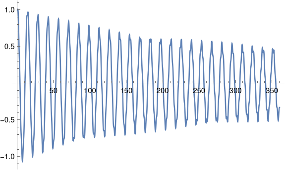
Here’s a plot of the solution as a function of time.

The solution basically looks like the solution of the linear case, except the solutions are more jagged near the local maxima and minima. In fact, the plot looks so jagged that I wondered whether this was an artifact of needing more plotting points. But adding more points didn’t make much difference. Interestingly, although this plot looks jagged, the phase portrait is smooth.

I produced the phase portrait by copying Trott’s code and making a couple small modifications.

    sol = NDSolve[{(*differential equation*)
        x''[t] + 1/20 x'[t]^3 + 1/5 x[t] == 
        1/3 Cos[E t],(*initial conditions*)x[0] == 1, x'[0] == 0}, 
        x, {t, 0, 360}, MaxSteps -> Infinity]

    ParametricPlot[Evaluate[{x[t], x'[t]} /. sol], {t, 0, 360}, 
        Frame -> True, Axes -> False, PlotPoints -> 3600]

Apparently the syntax of NDSolve has changed slightly since Trott’s book was published in 2004. The argument x in the code above was written x[t] in Trott’s original code and this did not work in the current version of Mathematica. I also simplified the call to ParametricPlot slightly, though the original code would work.

Predator-Prey period

The Lotka-Volterra equations are a system of nonlinear differential equations for modeling a predator-prey ecosystem. After a suitable change of units the equations can be written in the form
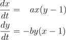
\begin{align*} \frac{dx}{dt} &= \phantom{-}ax(y-1) \\ \frac{dy}{dt} &= -by(x-1) \end{align}

where ab = 1. Here x(t) is the population of prey at time t and y(t) is the population of predators. For example, maybe x represents rabbits and y represents foxes, or x represents Eloi and y represents Morlocks.

It is well known that the Lotka-Volterra equations have periodic solutions. It is not as well known that you can compute the period of a solution without having to first solve the system of equations.

This post will show how to compute the period of the system. First we’ll find the period by solving the equations for a few different initial conditions, then we’ll show how to directly compute the period from the system parameters.

Phase plot

Here is a plot of (x(t), y(t)) showing that the solutions are periodic.
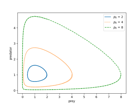
Predator-prey phase plots for varying initial conditions

And here’s the Python code that made the plot above.

    import matplotlib.pyplot as plt
    import numpy as np
    from scipy.integrate import solve_ivp
    
    # Lotka-Volterra equations
    def lv(t, z, a, b):
        x, y = z
        return [a*x*(y-1), -b*y*(x-1)]
    
    begin, end = 0, 20
    t = np.linspace(begin, end, 300)
    
    styles = ["-", ":", "--"]
    prey_init = [2, 4, 8]
    a = 1.5
    b = 1/a
    
    for style, p0 in zip(styles, prey_init):
        sol = solve_ivp(lv, [begin, end], [p0, 1], t_eval=t, args=(a, b))
        plt.plot(sol.y[0], sol.y[1], style)
    
    plt.xlabel("prey")
    plt.ylabel("predator")
    plt.legend([f"$p_0$ = {p0}" for p0 in prey_init])    

Note that the derivative of x is zero when y = 1. Since our initial condition sets y(0) = 1, we’re specifying the maximum value of x. (If our initial values of x were less than 1, we’d be specifying the minimum of x.)

Time plot

The components x and y have the same period, and that period depends on a and b, and on the initial conditions. The plot below shows how the period increases with x(0), which as we noted above is the maximum value of x.
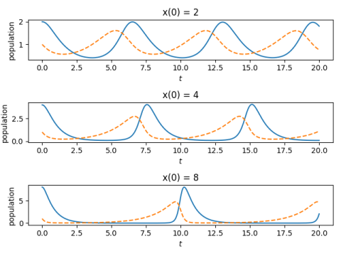
Predator-prey solutions over time for varying initial conditions

And here’s the code that made the plot.

    fig, ax = plt.subplots(3, 1)
    for i in range(3):
        sol = solve_ivp(lv, [begin, end], [prey_init[i], 1], t_eval=t, args=(a, b))
        ax[i].plot(t, sol.y[0], "-")
        ax[i].plot(t, sol.y[1], "--")    
        ax[i].set_xlabel("$t$")
        ax[i].set_ylabel("population")
        ax[i].set_title(f"x(0) = {prey_init[i]}")
    plt.tight_layout()

Finding the period

In [1] the author develops a way to compute the period of the system as a function of its parameters without solving the differential equations.

First, calculate an invariant h of the system:

h = b(x - \log(x) - 1) + a(y - \log(y) - 1)

Since this is an invariant we can evaluate it anywhere, so we evaluate it at the initial conditions.

Then the period only depends on a and h. (Recall we said we can scale the equations so that ab = 1, so a and b are not independent parameters.)

If h is not too large, we can compute the approximate period using an asymptotic series.

P(h) = 2\pi\left( 1 + \frac{\sigma}{6} h + \frac{\sigma^2}{144} h^2 + \left(\frac{\sigma}{360} - \frac{139\sigma^3}{38880}\right) h^3 + \cdots \right)

where σ = (a + b)/2 = (a² + 1)/2a.

We use this to find the periods for the example above.

    def find_h(a, x0, y0):
        b = 1/a
        return b*(x0 - np.log(x0) - 1) + a*(y0 - np.log(y0) - 1)

    def P(h, a):
        sigma = 0.5*(a + 1/a)
        s = 1 + sigma*h/6 + sigma**2*h**2/144
        return 2*np.pi*s

    print([P(find_h(1.5, p0, 1), 1.5) for p0 in [2, 4, 8]])

This predicts periods of roughly 6.5, 7.5, and 10.5, which is what we see in the plot above.

When h is larger, the period can be calculated by numerically evaluating an integral given in [1].

Related posts

[1] Jörg Waldvogel. The Period in the Volterra-Lotka Predator-Prey Model. SIAM Journal on Numerical Analysis, Dec., 1983, Vol. 20, No. 6, pp. 1264-1272


Oscillatory differential equations

The solution to a differential equation is called oscillatory if its set of zeros is unbounded. This does not necessarily mean that the solution is periodic, but that it crosses the horizontal axis infinitely often.

Fowler [1] studied the following differential equation demonstrates both oscillatory and nonoscillatory behavior.

x” + tσ |x|γ sgn x = 0

He proved that

  1. If σ + 2 ≥ 0 then all solutions oscillate.
  2. If σ + (γ + 3)/2 < 0 then no solutions oscillate.
  3. If neither (1) nor (2) holds then some solutions oscillate and some do not.

The edge case is σ = -2 and γ = 1. This satisfies condition (1) above. A slight decrease in σ will push the equation into condition (2). And a simultaneous decrease in σ and increase in γ can put it in condition (3).

It turns out that the edge case can be solved in closed form. The equation is linear because γ = 1 and solutions are given by

c √t sin(φ + √3 log(t) / 2).

The solutions oscillate because the argument to sine is an unbounded function of t, and so it runs across multiples of π infinitely often. The distance between zero crossings increases exponentially with time because the logarithms of the crossings are evenly spaced.

This post took a different turn after I started writing it. My original intention was to solve the differential equation numerically and say “See: when you change the parameters slightly you get what the theorem says.” But that didn’t work out.

First I tried numerically computing the solution above with σ = −2 and γ = 1, but I didn’t see oscillations. I tried making σ a little larger, but still didn’t see oscillations. When I increased σ more I could see the oscillations.

I was able to go back and see the oscillations with σ = −2 and γ = 1 by tweaking the parameters in my ODE solver. It’s best practice to tweak your parameters even if everything looks right, just to make sure your solution is robust to algorithm changes. Maybe I would have done that, but since I already knew the analytic solution, I knew to tweak the parameters until I saw the right behavior.

Without some theory as a guide, it would be difficult to determine from numerical solutions alone whether a solution oscillates. If you see oscillations, then they’re probably real (unless your numerical method is unstable), but if you don’t see oscillations, how do you know you won’t see them if you look further out? How much further out should you look? In a practical application, the context of your problem will tell you how far out to look.

My intention was to recommend the equation above as an illustration for an introductory DE class because it demonstrates the important fact that small changes to an equation can qualitatively change the behavior of the solutions. This is especially true for nonlinear DEs, which the above equation is when γ ≠ 1. It could still be used for that purpose, but it would make a better demonstration than homework exercise. The instructor could tune the DE solver to make sure the solutions are qualitatively correct.

I recommend the equation as an illustration, but for a course covering numerical solutions to DEs. It illustrates a different point than I first intended, namely the potentially finicky behavior of software for solving differential equations.

There are a couple morals to this story. One is that numerical methods have not eliminated the need for theory. The ideal is to combine analytic and numerical methods. Analytic methods point out qualitative behavior that might be hard to discover numerically. And analytic methods are not likely to produce closed-form solutions for nonlinear DEs.

Another moral is that it’s best to twiddle the parameters to your numerical method to make sure the solution doesn’t qualitatively change. If you’ve adequately computed a solution, computing it again with smaller integration steps shouldn’t make much difference. But if you do see a substantial difference, your first solution probably wasn’t as good as you thought.

Related posts

[1] R. H. Fowler. Further studies of Emden’s and similar differential equations. Quarterly Journal of Mathematics. 2 (1931), pp. 259–288.

Laplacian in various coordinate systems

The recent post on the wave equation on a disk showed that the Laplace operator has a different form in polar coordinates than it does in Cartesian coordinates. In general, the Laplacian is not simply the sum of the second derivatives with respect to each variable.

Mathematica has a function, unsurprisingly called Laplacian, that will compute the Laplacian of a given function in a given coordinate system. If you give it a specific function, it will compute the Laplacian of that function. But you can also give it a general function to find a general formula.

For example,

    Simplify[Laplacian[f[r, θ], {r, θ}, "Polar"]]

returns

\frac{f^{(0,2)}(r,\theta )}{r^2}+\frac{f^{(1,0)}(r,\theta )}{r}+f^{(2,0)}(r,\theta )

This is not immediately recognizable as the Laplacian from this post

\Delta u = \frac{\partial^2 u}{\partial r^2} + \frac{1}{r} \frac{\partial u}{\partial r} + \frac{1}{r^2} \frac{\partial^2 u}{\partial \theta^2}

because Mathematica is using multi-index notation, which is a little cumbersome for simple cases, but much easier to use than classical notation when things get more complicated. The superscript (0,2), for example, means do not differentiate with respect to the first variable and differentiate twice with respect to the second variable. In other words, take the second derivative with respect to θ.

Here’s a more complicated example with oblate spheroidal coordinates. Such coordinates come in handy when you need to account for the fact that our planet is not exactly spherical but is more like an oblate spheroid.

When we ask Mathematica

    Simplify[Laplacian[f[ξ, η, φ], {ξ, η, φ}, "OblateSpheroidal"]]

the result isn’t pretty.

(Csc[\[Eta]]^2*Sech[\[Xi]]^2*Derivative[0, 0, 2][f][\[Xi], \[Eta], \[Phi]] + (2*(Cot[\[Eta]]*Derivative[0, 1, 0][f][\[Xi], \[Eta], \[Phi]] + Derivative[0, 2, 0][f][\[Xi], \[Eta], \[Phi]] + Tanh[\[Xi]]*Derivative[1, 0, 0][f][\[Xi], \[Eta], \[Phi]] + Derivative[2, 0, 0][f][\[Xi], \[Eta], \[Phi]]))/ (Cos[2*\[Eta]] + Cosh[2*\[Xi]]))/\[FormalA]^2

I tried using TeXForm and editing it into something readable, but after spending too much time on this I gave up and took a screenshot. But as ugly as the output is, it would be uglier (and error prone) to do by hand.

Mathematica supports the following 12 coordinate systems in addition to Cartesian coordinates:

  • Cylindrical
  • Bipolar cylindrical
  • Elliptic cylindrical
  • Parabolic cylindrical
  • Circular parabolic
  • Confocal paraboloidal
  • Spherical
  • Bispherical
  • Oblate spheroidal
  • Prolate spheroidal
  • Conical
  • Toroidal

These are all orthogonal, meaning that surfaces where one variable is held constant meet at right angles. Most curvilinear coordinate systems used in practice are orthogonal because this simplifies a lot of things.

Laplace’s equation is separable in Stäckel coordinate systems. These are all these coordinate systems except for toroidal coordinates. And in fact Stäckel coordinates are the only coordinate systems in which Laplace’s equation is separable.

It’s often the case that Laplace’s equation is separable in orthogonal coordinate systems, but not always. I don’t have a good explanation for why toroidal coordinates are an exception.

If you’d like a reference for this sort of thing, Wolfram Neutsch’s tome Coordinates is encyclopedic. However, it’s expensive new and hard to find used.

Vibrating circular membranes

'Snare drum' by YannickWhee is licensed under CC BY 2.0

This post will tie together many things I’ve blogged about before. The previous post justified separation of variables. This post will illustrate separation of variables.

Also, this post will show why you might care about Bessel functions and their zeros. I’ve written about Bessel functions before, and said that Bessel functions are to polar coordinates what sines and cosines are to rectangular coordinates. This post will make this analogy more concrete.

Separation of variables

The separation of variables technique is typically presented in three contexts in introductory courses on differential equations:

  1. One-dimensional heat equation
  2. One-dimensional wave equation
  3. Two-dimensional (rectangular) Laplace equation

My initial motivation for writing this post was to illustrate separation of variables outside the most common examples. Separation of variables requires PDEs to have a special form, but not as special as the examples above might imply. A secondary motivation was to show Bessel functions in action.

Radially symmetric wave equation

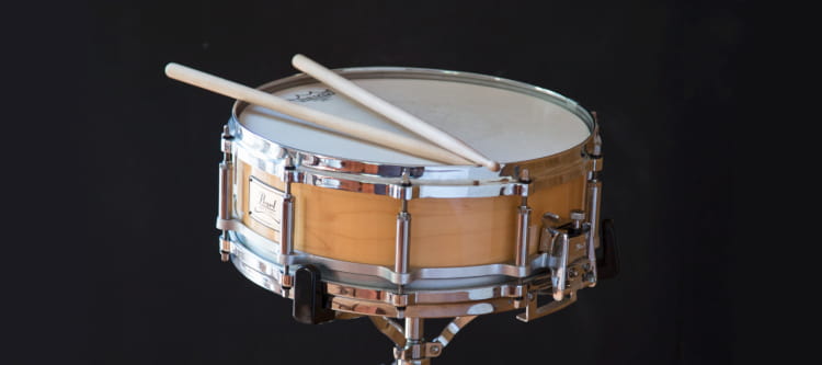
Suppose you have a thin membrane, like a drum head, and you want to model its vibrations. By “thin” I mean that the membrane is sufficiently thin that we can adequately model it as a two-dimensional surface bobbing up and down in three dimensions. It’s not so thick that we need to model the material in more detail.

Let u(x, y, t) be the height of the membrane at location (x, y) and time t. The wave equation is a PDE modeling the motion of the membrane by

\frac{\partial^2 u}{\partial t^2} = c^2 \Delta u. width=

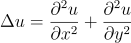
where Δ is the Laplacian operator. In rectangular coordinates the Laplacian is given by

\Delta u = \frac{\partial^2 u}{\partial x^2} + \frac{\partial^2 u}{\partial y^2}
We’re interested in a circular membrane, and so things will be much easier if we work in polar coordinates. In polar coordinates the Laplacian is given by

\Delta u = \frac{\partial^2 u}{\partial r^2} + \frac{1}{r} \frac{\partial u}{\partial r} + \frac{1}{r^2} \frac{\partial^2 u}{\partial \theta^2}

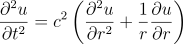
We will assume that our boundary conditions and initial conditions are radially symmetric, and so our solution will be radially symmetric, i.e. derivatives with respect to θ are zero. And in our case the wave equation simplifies to

\frac{\partial^2 u}{\partial t^2} = c^2 \left( \frac{\partial^2 u}{\partial r^2} + \frac{1}{r} \frac{\partial u}{\partial r} \right)

Boundary and initial conditions

Let a be the radius of our membrane. We will assume our membrane is clamped down on its boundary, like a drum head, which means we have the boundary condition

u(a, t) = 0

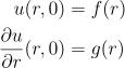
for all t ≥ 0. We assume the initial displacement and initial velocity of the membrane are given by

\begin{align*} u(r, 0) &= f(r) \\ \frac{\partial u}{\partial r}(r, 0) &= g(r) \end{align*}

for all r between 0 and a.

Separating variables

Now we get down to separation of variables. Because we’re assuming radial symmetry, we’re down to a function of two variables: r for the distance from the center and t for time. We assume

u(r, t) = R(r) T(t)

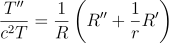
and stick it into the wave equation. A little calculation shows that

\frac{T''}{c^2 T} = \frac{1}{R} \left(R'' + \frac{1}{r} R'\right)

The left side is a function of t alone, and the right side is a function of r alone. The only way this can be true for all t and all r is for both sides to be constant. Call this constant -λ². Why? Because looking ahead a little we find that this will make things easier shortly.

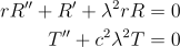
Separation of variables allowed us to reduce our PDE to the following pair of ODEs.

r R'' + R' +\lambda^2 r R &= 0 \\ T'' + c^2 \lambda^2 T &= 0

The solutions to the equation for R are linear combinations of the Bessel functions J0(λr) and Y0(λr) [1].

And the solutions to the equation for T are linear combinations of the trig functions cos(cλt) and sin(cλt).

The boundary condition u(a, t) = 0 implies the boundary condition R(a) = 0. This implies that λa must be a zero of our Bessel function, and that all the Y0 terms drop out. This means that our solution is

u(r,t) = \sum_{n=1}^\infty J_0(\lambda_n r) \left( A_n \cos(c \lambda_n t) + B_n \sin(c \lambda_n t)\right)

where

\lambda_n = \frac{\alpha_n}{a}.

Here αn are the zeros of the Bessel function J0.

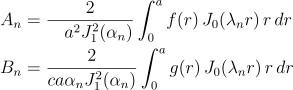
The coefficients An and Bn are determined by the initial conditions. Specifically, you can show that

\begin{align*} A_n &= \frac{2}{\phantom{ca}a^2 J_1^2(\alpha_n)} \int_0^a f(r)\, J_0(\lambda_n r) \, r\, dr \\ B_n &= \frac{2}{ca \alpha_n J_1^2(\alpha_n)} \int_0^a g(r)\, J_0(\lambda_n r) \, r\, dr \\ \end{align*}

The function J1 in the expression for the coefficients is another Bessel function.

The functions J0 and J1 are so important in applications that even the otherwise minimalist Unix calculator bc includes these functions. (As much as I appreciate Bessel functions, this still seems strange to me.) And you can find functions for zeros of Bessel functions in many libraries, such as scipy.special.jn_zeros in Python.

Related posts

[1] This is why introductory courses are unlikely to include an example in polar coordinates. Separation of variables itself is no harder in polar coordinates than in rectangular coordinates, and it shows the versatility of the method to apply it in a different setting.

But the resulting ODEs have Bessel functions for solutions, and it’s understandable that an introductory course might not want to go down this rabbit trail, especially since PDEs are usually introduced at the end of a differential equation class when professors are rushed and students are tired.

[2] Snare drum image above “Snare drum” by YannickWhee is licensed under CC BY 2.0

Justifying separation of variables

The separation of variables technique for solving partial differential equations looks like a magic trick the first time you see it. The lecturer, or author if you’re more self-taught, makes an audacious assumption, like pulling a rabbit out of a hat, and it works.

For example, you might first see the heat equation

ut = c² uxx.

The professor asks you to assume the solution has the form

u(x, t) = X(x) T(t).

i.e. the solution can be separated into the product of a function of x alone and a function of t alone.

Following that you might see Laplace’s equation on a rectangle

uxx + uyy = 0

with the analogous assumption that

u(x, y) = X(x) Y(y),

i.e. the product of a function of x alone and a function of y alone.

There are several possible responses to this assumption.

  1. Whatever you say, doc.
  2. How can you assume that?
  3. How do you know you’re not missing any possibilities?
  4. What made someone think to try this?

As with many things, separation of variables causes the most consternation for the moderately sophisticated students. The least sophisticated students are untroubled, and the most sophisticated student can supply their own justification (at least after the fact).

One response to question (2) is “Bear with me. I’ll show that this works.”

Another response would be “OK, how about assuming the solution is a sum of such functions. That’s a much larger space to look in. And besides, we are going to take sums of such solutions in a few minutes.” One could argue from functional analysis or approximation theory that the sums of separable functions are dense in reasonable space of functions [1].

This is a solid explanation, but it’s kind of anachronistic: most students see separation of variables long before they see functional analysis or approximation theory. But it would be a satisfying response for someone who is seeing all this for the second time. Maybe they were exposed to separation of variables as an undergraduate and now they’re taking a graduate course in PDEs. In an undergraduate class a professor could do a little foreshadowing, giving the students a taste of approximation theory.

Existence of solutions is easier to prove than uniqueness in this case because you can concretely construct a solution. This goes back to the “it works” justification. This argument deserves more respect than a sophomoric student might give it. Mathematics research is not nearly as deductive and mathematics education. You often have to make inspired guesses and then show that they work.

Addressing question (3) requires saying something about uniqueness. A professor could simply assert that there are uniqueness theorems that allow you to go from “I’ve found something that works” to “and so it must be the only thing that works.” Or one could sketch a uniqueness theorem. For example, you might apply a maximum principle to show that the difference between any two solutions is zero.

Question (4) is in some sense the most interesting question. It’s not a mathematical question per se but a question about how people do mathematics. I don’t know what was going through the mind of the first person to try separation of variables, or even who this person was. But a plausible line of thinking is that ordinary differential equations are easier than partial differential equations. How might you reduce a PDE to an ODE? Well, if the solution could be factored into functions of one variable, …

The next post will illustrate using separation of variables by solving the wave equation on a disk.

Related posts

[1] Also, there’s the mind-blowing Kolmogorov-Arnol’d theorem. This theorem says any continuous function of several variables can be written as a sum of continuous separable functions. It doesn’t say you can make the functions in your sum smooth, but it suggests that sums of separable functions are more expressive than you might have imagined.

Fourier, Gauss, and Heisenberg

Several weeks ago I wrote about the Fourier uncertainty principle which gives a lower bound on the product of the variance of a function f and the variance of its Fourier transform. This post expands on the earlier post by quoting some results from a recent paper [1].

Gaussian density

The earlier post said that the inequality in the Fourier uncertainty principle is exact when f is proportional to a Gaussian probability density. G. H. Hardy proved this result in 1933 in the form of the following theorem.

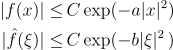
Let f be a square-integrable function on the real line and assume f and its Fourier transform satisfy the following bounds

\begin{align*} |f(x)| \leq& \,C \exp(-a|x|^2) \\ |\hat{f}(\xi)| \leq& \,C \exp(-b|\xi|^2\,) \\ \end{align*}

for some constant C. Then if ab > 1/4, then f = 0. And if ab = 1/4, f(x) = c exp(−ax²) for some constant c.

Let’s translate this into probability terms by setting

\begin{align*} a =& \,\frac{1}{2\sigma^2} \\ b =& \,\frac{1}{2\tau^2} \end{align*}

Now Hardy’s theorem says that if f is bounded by a multiple of a Gaussian density with variance σ² and its Fourier transform is bounded by a multiple of a Gaussian density with variance τ², then the product of the two variances is no greater than 1. And if the product of the variances equals 1, then f is a multiple of a Gaussian density with variance σ².

Heisenberg uncertainty

Theorem 3 in [1] says that if u(t, x) is a solution to the free Schrödinger’s equation

\partial_t u = i \Delta u

then u at different points in time satisfies a theorem similar to Hardy’s theorem. In fact, the authors show that this theorem is equivalent to Hardy’s theorem.

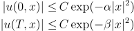
Specifically, if u is a sufficiently smooth solution and

\begin{align*} |u(0,x)| \leq& \,C \exp(-\alpha|x|^2) \\ |u(T,x)| \leq& \,C \exp(-\beta|x|^2) \\ \end{align*}

then αβ > (4T)−2 implies u(t, x) = 0, and αβ = (4T)−2 implies

u(t,x) = c \exp(-(\alpha + i/(4T))|x|^2)

Related posts

[1] Aingeru Fernández-Bertolin and Eugenia Malinnikova. Dynamical versions of Hardy’s uncertainty principle: A survey. Bulletin of the American Mathematical Society. DOI: https://doi.org/10.1090/bull/1729