Scaled Beta2 distribution

I recently ran across a new probability distribution called the “Scaled Beta2” or “SBeta2” for short in [1].

For positive argument x and for positive parameters p, q, and b, its density is

\frac{\Gamma(p+q)}{b\,\Gamma(p) \, \Gamma(q)}\, \frac{\left(\frac{x}{b}\right)^{p-1}}{\left(\left(\frac{x}{b}\right) + 1 \right)^{p+q}}

This is a heavy-tailed distribution. For large x, the probability density is O(xq−1), the same as a Student-t distribution with q degrees of freedom.

The authors in [1] point out several ways this distribution can be useful in application. It can approximate a number of commonly-used prior distributions while offering advantages in terms of robustness and analytical tractability.

Related posts

[1] The Scaled Beta2 Distribution as a Robust Prior for Scales. María-Eglée Pérez, Luis Raúl Pericchi, Isabel Cristina Ramírez. Available here.

Fraction comparison trick

If you want to determine whether

a/b > c/d,

it is often enough to test whether

a + d > b + c.

Said another way a/b is usually greater than c/d when a + d is greater than b + c.

This sounds imprecise if not crazy. But it is easy to make precise and [1] shows that it is true.

Examples

Consider 4/11 vs 3/7. In this case 4 + 7 = 11 < 11 + 3 = 14, which suggests 4/11 < 3/7, which is correct.

But the rule of thumb can lead you astray. For example, suppose you want to compare 3/7 and 2/5. We have 3 + 5 = 8 < 7 + 2 = 9, but 3/7 > 2/5.

The claim isn’t that the rule always works; clearly it doesn’t. The claim is that it usually works, in a sense that will be made precise in the next section.

Rigorous statement

Let N be a large integer, and pick integers a, b, c, and d at random uniformly between 1 and N. Let

x = a/bc/d

and

y = (a+d) − (b+c).

Then the probability x and y are both positive, or both negative, or both zero, approaches 11/12 as N goes to infinity.

Simulation

I won’t repeat the proof of the theorem above; see [1] for that. But I’ll give a simulation that illustrates the theorem.

    import numpy as np
    
    np.random.seed(20210225)
    
    N = 1_000_000
    numreps = 10_000
    
    count = 0
    for _ in range(numreps):
        (a, b, c, d) = np.random.randint(1, N+1, 4, dtype=np.int64)
        x = a*d - b*c
        y = (a+d) - (b+c)
        if np.sign(x) == np.sign(y):
            count += 1
    print(count/numreps)

This prints 0.9176, and 11/12 = 0.91666….

The random number generator randint defaults to 32-bit integers, but this could lead to overflow since 106 × 106 > 232. So I used 64-bit integers.

Instead of computing a/bc/d, I multiply by bd and compute adbc instead because this avoids any possible floating point issues.

In case you’re not familiar with the sign function, it returns 1 for positive numbers, 0 for 0, and −1 for negative numbers.

The code suggests a different statement of the theorem: if you generate two pairs of integers, their sums and their products are probably ordered the same way.

Psychology

This post has assumed that the numbers a, b, c, and d are all chosen uniformly at random. But the components of the fractions for which you have any doubt whether a/b is greater or less than c/d are not uniformly distributed. For example, consider 17/81 versus 64/38. Clearly the former is less than 1 and the latter is greater than 1.

It would be interesting to try to assess how often the rule of thumb presented here is correct in practice. You might try to come up with a model for the kinds of fractions people can’t compare instantly, such as proper fractions that have similar size.

Related posts

[1] Kenzi Odani. A Rough-and-Ready Rule for Fractions. The Mathematical Gazette, Vol. 82, No. 493 (Mar., 1998), pp. 107-109

Normal probability fixed point

Let Z be a standard normal random variable. Then there is a unique x such that

Pr(Z < x) = x.

That is, Φ has a unique fixed point where Φ is the CDF of a standard normal.

It’s easy to find the fixed point: start anywhere and iterate Φ.

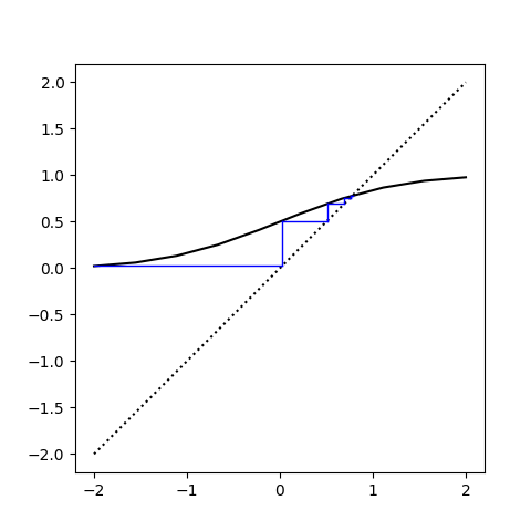
Here’s a cobweb plot that shows how the iterates converge, starting with −2.

Cobweb plot for normal CDF

The black curve is a plot of Φ. The blue stairstep is a visualization of the iterates. The stairstep pattern comes from outputs turning into inputs. That is, vertical blue lines connect and input value x to its output value y, and the horizontal blue lines represent sliding a y value over to the dotted line y = x in order to turn it into the next x value.

y‘s become x‘s. The blue lines get short when we’re approaching the fixed point because now the outputs approximately equal the inputs.

Here’s a list of the first 10 iterates.

    0.02275
    0.50907
    0.69465
    0.75636
    0.77528
    0.78091
    0.78257
    0.78306
    0.78320
    0.78324

So it seems that after 10 iterations, we’ve converged to the fixed point in the first four decimal places.

Random polynomials revisited

A few days ago I wrote about the expected number of roots in a random polynomial where each coefficient is drawn from a standard normal, i.e. a Gaussian distribution with mean 0 and variance 1.

Another class of random polynomials, one that comes up in applications to physics, draws each coefficient from a different distribution. Specifically, the nth coefficient in an Nth degree polynomial is drawn from a normal distribution with mean zero and variance N choose n. As before, our reference is [1].

It turns out that for these random polynomials, the expected number of real zeros is √N. This is not an asymptotic approximation.

For an example, I created a random 44th degree polynomial.

    from scipy.stats import norm
    from scipy.special import binom

    N = 44
    coeff = [norm.rvs(scale=binom(N,n)**0.5) for n in range(N+1)]

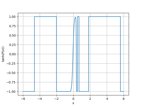
I plotted the (tanh of) this polynomial as described here.

This polynomial clearly has 8 real roots. The expected number of roots for a 44th degree random polynomial of this type is √44 = 6.63.

[1] Alan Edelman and Eric Kostlan. How many zeros of a random polynomial are real? Bulletin of the AMS. Volume 32, Number 1, January 1995

Large matrices rarely have saddlepoints

A matrix is said to have a saddlepoint if an element is the smallest element in its row and the largest element in its column. For example, 0.546 is a saddlepoint in the matrix below because it is the smallest element in the third row and the largest element in the first column.

\begin{bmatrix} -0.850 & 1.529 & \phantom{-}0.896 \\ -1.878 & 1.233 & -0.200 \\ \phantom{-}0.546 & 0.762 & \phantom{-}1.763 \\ -0.449 & 3.136 & \phantom{-}1.345 \end{bmatrix}

In [1], Goldman considers the probability of an m by n matrix having a saddlepoint if its elements are chosen independently at random from the same continuous distribution. He reports this probability as

\frac{m!\,\,n!}{(m+n-1)!}

but it may be easier to interpret as

\left. (m+n) \middle/ {m+n \choose n} \right.

When m and n are large, the binomial coefficient in the denominator is very large.

For square matrices, m and n are equal, and the probability above is 2n/(n + 1) divided by the nth Catalan number Cn.

A couple years ago I wrote about bounds on the middle binomial coefficient

\frac{2^{2n-1}}{\sqrt{n}} < \binom{2n}{n} < \frac{2^{2n-1/2}}{\sqrt{n}}

by E. T. H. Wang. These bounds let us conclude that P(n, n), the probability of an n by n matrix having a saddlepoint, is bounded as follows.

\frac{n^{3/2}}{2^{2n - 3/2}} < P(n,n) < \frac{n^{3/2}}{2^{2n-2}}

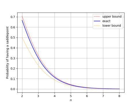
Here’s a plot of P(n, n) and its bounds.

plot of saddlepoint probability and its bounds

This shows that the probability goes to zero exponentially as n increases, being impossible to visually distinguish from 0 in the plot above when n = 8.

The upper bound on P(n, n) based on Wang’s inequalities is tighter than the corresponding lower bound. This is because Wang’s lower bound on the middle binomial coefficient is tighter (see plot here) and we’ve taken reciprocals.

Simulation

The theory above says that if we generate 4 by 3 matrices with independent normal random values, each matrix with have a saddle point with probability 1/5. The following code generates 10,000 random 4 by 3 matrices and counts what proportion have a saddle point.

    
    import numpy as np
    from scipy.stats import norm

    def has_saddlepoint(M):
        m, n = M.shape
        row_min_index = [np.argmin(M[i,:]) for i in range(m)]
        col_max_index = [np.argmax(M[:,j]) for j in range(n)]
        for i in range(m):
            if col_max_index[row_min_index[i]] == i:
                return True
        return False

    m, n = 4, 3
    N = 10000
    saddlepoints = 0

    for _ in range(N):
        M = norm.rvs(size=(m,n))
        if has_saddlepoint(M):
            saddlepoints += 1
    print(saddlepoints / N)

When I ran this, I got 0.1997, very close to the expected value.

More on random matrices

[1] A. J. Goldman. The Probability of a Saddlepoint. The American Mathematical Monthly, Vol. 64, No. 10, pp. 729-730

Informative stopping

When the rule for stopping an experiment depends on the data in the experiment, the results could be biased if the stopping rule isn’t taken into account in the analysis [1].

For example, suppose Alice wants to convince Bob that π has a greater proportion of even digits than odd digits.

Alice: I’ll show you that π has more even digits than odd digits by looking at the first N digits. How big would you like N to be?

Bob: At least 1,000. Of course more data is always better.

Alice: Right. And how many more even than odd digits would you find convincing?

Bob: If there are at least 10 more evens than odds, I’ll believe you.

Alice: OK. If you look at the first 2589 digits, there are 13 more even digits than odd digits.

Now if Alice wanted to convince Bob that there are more odd digits, she could do that too. If you look at the first 2077 digits, 13 more are odd than even.

No matter what two numbers Bob gives, Alice can find a sample size that will give the result she wants. Here’s Alice’s Python code.

    from mpmath import mp
    import numpy as np

    N = 3000 
    mp.dps = N+2
    digits = str(mp.pi)[2:]

    parity = np.ones(N, dtype=int)
    for i in range(N):
        if digits[i] in ['1', '3', '5', '7', '9']:
            parity[i] = -1
    excess = parity.cumsum()
    print(excess[-1])
    print(np.where(excess == 13))
    print(np.where(excess == -13))

The number N is a guess at how far out she might have to look. If it doesn’t work, she increases it and runs the code again.

The array parity contains a 1 in positions where the digits of π (after the decimal point) are even and a -1 where they are odd. The cumulative sum shows how many more even than odd digits there have been up to a given point, a negative number meaning there have been more odd digits.

Alice thought that stopping when there are exactly 10 more of the parity she wants would look suspicious, so she looked for places where the difference was 13.

Here are the results:

    [ 126,  128,  134,  …,  536, 2588, … 2726]
    [ 772,  778,  780,  …,  886, 2076, … 2994]

There’s one minor gotcha. The array excess is indexed from zero, so Alice reports 2589 rather than 2588 because the 2589th digit has index 2588.

Bob’s mistake was that he specified a minimum sample size. By saying “at least 1,000” he gave Alice the freedom to pick the sample size to get the result she wanted. If he specified an exact sample size, there probably would be either more even digits or more odd digits, but there couldn’t be both. And if he were more sophisticated enough, he could pick an excess value that would be unlikely given that sample size.

Related posts

[1] This does not contradict the likelihood principle; it says that informative stopping rules should be incorporated into the likelihood function.

Random Fibonacci numbers

The Fibonacci numbers are defined by F1 = F2 = 1, and for n > 2,

Fn = Fn-1 + Fn-2.

A random Fibonacci sequence f is defined similarly, except the addition above is replaced with a subtraction with probability 1/2. That is, f1 = f2 = 1, and for n > 2,

fn = fn-1 + b fn-2

where b is +1 or -1, each with equal probability.

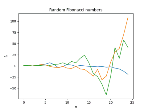
Here’s a graph a three random Fibonacci sequences.

Graph of random Fibonacci sequences

Here’s the Python code that was used to produce the sequences above.

    import numpy as np

    def rand_fib(length):
        f = np.ones(length)
        for i in range(2, length):
            b = np.random.choice((-1,1))
            f[i] = f[i-1] + b*f[i-2]
        return f

It’s easy to see that the nth random Fibonacci number can be as large as the nth ordinary Fibonacci number if all the signs happen to be positive. But the numbers are typically much smaller.

The nth (ordinary) Fibonacci number asymptotically approaches φn is the golden ratio, φ = (1 + √5)/2 = 1.618…

Another way to say this is that

\lim_{n\to\infty}(F_n)^{1/n} = \varphi

The nth random Fibonacci number does not have an asymptotic value—it wanders randomly between positive and negative values—but with probability 1, the absolute values satisfy

\lim_{n\to\infty}|f_n|^{1/n} = 1.1319882\ldots

This was proved in 1960 [1].

Here’s a little Python code to show that we get results consistent with this result using simulation.

    N = 500
    x = [abs(rand_fib(N)[-1])**(1/N) for _ in range(10)]
    print(f"{np.mean(x)} ± {np.std(x)}")

This produced

1.1323 ± 0.0192

which includes the theoretical value 1.1320.

Update: The next post looks at whether every integer appear in a random Fibonacci sequence. Empirical evidence suggests the answer is yes.

Related posts

[1] Furstenberg and Kesten. Products of random matrices. Ann. Math. Stat. 31, 457-469.

Real-time analytics

There’s an ancient saying “Whom the gods would destroy they first make mad.” (Mad as in crazy, not mad as in angry.) I wrote a variation of this on Twitter:

Whom the gods would destroy, they first give real-time analytics.

Having more up-to-date information is only valuable up to a point. Past that point, you’re more likely to be distracted by noise. The closer you look at anything, the more irregularities you see, and the more likely you are to over-steer [1].

I don’t mean to imply that the noise isn’t real. (More on that here.) But there’s a temptation to pay more attention to the small variations you don’t understand than the larger trends you believe you do understand.

I became aware of this effect when simulating Bayesian clinical trial designs. The more often you check your stopping rule, the more often you will stop [2]. You want to monitor a trial often enough to shut it down, or at least pause it, if things change for the worse. But monitoring too often can cause you to stop when you don’t want to.

Flatter than glass

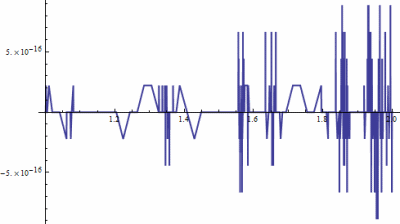
A long time ago I wrote about the graph below.

The graph looks awfully jagged, until you look at the vertical scale. The curve represents the numerical difference between two functions that are exactly equal in theory. As I explain in that post, the curve is literally smoother than glass, and certainly flatter than a pancake.

Notes

[1] See The Logic of Failure for a discussion of how over-steering is a common factor in disasters such as the Chernobyl nuclear failure.

[2] Bayesians are loathe to talk about things like α-spending, but when you’re looking at stopping frequencies, frequentist phenomena pop up.

Sample size calculation

If you’re going to run a test on rabbits, you have to decide how many rabbits you’ll use. This is your sample size. A lot of what statisticians do in practice is calculate sample sizes.

A researcher comes to talk to a statistician. The statistician asks what effect size the researcher wants to detect. Do you think the new thing will be 10% better than the old thing? If so, you’ll need to design an experiment with enough subjects to stand a good chance of detecting a 10% improvement. Roughly speaking, sample size is inversely proportional to the square of effect size. So if you want to detect a 5% improvement, you’ll need 4 times as many subjects as if you want to detect a 10% improvement.

You’re never guaranteed to detect an improvement. The race is not always to the swift, nor the battle to the strong. So it’s not enough to think about what kind of effect size you want to detect, you also have to think about how likely you want to be to detect it.

Here’s what often happens in practice. The researcher makes an arbitrary guess at what effect size she expects to see. Then initial optimism may waver and she decides it would be better to design the experiment to detect a more modest effect size. When asked how high she’d like her chances to be of detecting the effect, she thinks 100% but says 95% since it’s necessary to tolerate some chance of failure.

The statistician comes back and says the researcher will need a gargantuan sample size. The researcher says this is far outside her budget. The statistician asks what the budget is, and what the cost per subject is, and then the real work begins.

The sample size the negotiation will converge on is the budget divided by the cost per sample. The statistician will fiddle with the effect size and probability of detecting it until the inevitable sample size is reached. This sample size, calculated to 10 decimal places and rounded up to the next integer, is solemnly reported with a post hoc justification containing no mention of budgets.

Sample size is always implicitly an economic decision. If you’re willing to make it explicitly an economic decision, you can compute the expected value of an experiment by placing a value on the possible outcomes. You make some assumptions—you always have to make assumptions—and calculate the probability under various scenarios of reaching each conclusion for various sample sizes, and select the sample size that leads to the best expected value.

More on experimental design

[1] There are three ways an A/B test can turn out: A wins, B wins, or there isn’t a clear winner. There’s a tendency to not think enough about the third possibility. Interim analysis often shuts down an experiment not because there’s a clear winner, but because it’s becoming clear there is unlikely to be a winner.

Truncated distributions vs clipped distributions

In the previous post, I looked at truncated probability distributions. A truncated normal distribution, for example, lives on some interval and has a density proportional to a normal distribution; the proportionality constant is whatever it has to be to make the density integrate to 1.

Truncated distributions

Suppose you wanted to generate random samples from a normal distribution truncated to [a, b]. How would you go about it? You could generate a sample x from the (full) normal distribution, and if axb, then return x. Otherwise, try again. Keep trying until you get a sample inside [a, b], and when you get one, return it [1].

This may be the most efficient way to generate samples from a truncated distribution. It’s called the accept-reject method. It works well if the probability of a normal sample being in [a, b] is high. But if the interval is small, a lot of samples may be rejected before one is accepted, and there are more efficient algorithms. You might also use a different algorithm if you want consistent run time more than minimal average run time.

Clipped distributions

Now consider a different kind of sampling. As before, we generate a random sample x from the full normal distribution and if axb we return it. But if x > b we return b. And if x < a we return a. That is, we clip x to be in [a, b]. I’ll call this a clipped normal distribution. (I don’t know whether this name is standard, or even if there is a standard name for this.)

Clipped distributions are not truncated distributions. They’re really a mixture of three distributions. Start with a continuous random variable X on the real line, and let Y be X clipped to [a, b]. Then Y is a mixture of a continuous distribution on [a, b] and two point masses: Y takes on the value a with probability P(X < a) and Y takes on the value b with probability P(X > b).

Clipped distributions are mostly a nuisance. Maybe the values are clipped due to the resolution of some sensor: nobody wants to clip the values, that’s just a necessary artifact. Or maybe values are clipped because some form only allows values within a given range; maybe the person designing the form didn’t realize the true range of possible values.

It’s common to clip extreme data values while deidentifying data to protect privacy. This means that not only is some data deliberately inaccurate, it also means that the distribution changes slightly since it’s now a clipped distribution. If that’s unacceptable, there are other ways to balance privacy and statistical utility.

Related posts

[1] Couldn’t this take forever? Theoretically, but with probability zero. The number of attempts follows a geometric distribution, and you could use that to find the expected number of attempts.