SymPy book

There’s a new book on SymPy, a Python library for symbolic math.

The book is Instant SymPy Starter by Ronan Lamy. As far as I know, this is the only book just on SymPy. It’s only about 50 pages, which is nice. It’s not a replacement for the online documentation but just a quick start guide.

The online SymPy documentation is good, but I think it would be easier to start with this book. And although I’ve been using SymPy off and on for a while, I learned a few things from the book.

Need a 12-digit prime?

You may have seen the joke “Enter any 12-digit prime number to continue.” I’ve seen it floating around as the punchline in several contexts.

So what do you do if you need a 12-digit prime? Here’s how to find the smallest one using Python.

    >>> from sympy import nextprime
    >>> nextprime(10**11)
    100000000003L

The function nextprime gives the smallest prime larger than its argument. (Note that the smallest 12-digit number is 1011, not 1012. Great opportunity for an off-by-one mistake.)

Optionally you can provide an addition argument to nextprime to get primes further down the list. For example, this gives the second prime larger than 1011.

    >>> nextprime(10**11, 2)
    100000000019L

What if you wanted the largest 12-digit prime rather than the smallest?

    >>> from sympy import prevprime
    >>> prevprime(10**12)
    999999999989L

Finally, suppose you want to know how many 12-digit primes there are. SymPy has a function primepi that returns the number of primes less than its argument. Unfortunately, it fails for large arguments. It works for arguments as big as 2**27 but throws a memory error for 2**28.

The number of primes less than n is approximately n / log n, so there are about 32 billion primes between 1011 and 1012. According to Wolfram Alpha, the exact number of 12-digit primes is 33,489,857,205. So if you try 12-digit numbers at random, your chances are about 1 in 30 of getting a prime. If you’re clever enough to just pick odd numbers, your chances go up to 1 in 15.

Synchronizing cicadas with Python

Suppose you want to know when your great-grandmother was born. You can’t find the year recorded anywhere. But you did discover an undated letter from her father that mentions her birth and one curious detail:  the 13-year and 17-year cicadas were swarming.

You do a little research and find that the 13-year cicadas are supposed to come out next year, and that the 17-year cicadas came out last year. When was your great-grandmother born?

Since 13 and 17 are relatively prime, the 13-year and 17-year cicadas will synchronize their schedules every 13 × 17 = 221 years. Suppose your great-grandmother was born n years ago. The remainder when n is divided by 13 must be 12, and the remainder when n is divided by 17 must be 1. We have to solve the pair of congruences n = 12 mod 13 and n = 1 mod 17. The Chinese Remainder Theorem says that this pair of congruences has a solution, and the proof of the theorem suggests an algorithm for computing the solution.

The Python library SymPy has a function for solving linear congruences.

    >>> from sympy.ntheory.modular import solve_congruence
    >>> solve_congruence( (12, 13), (1, 17) )
    (103, 221)

This says we’re 103 years into the joint cycle of the 13-year and 17-year cicadas. So your great-grandmother was born 103 years ago. (The solution 324 = 103 + 221 is also mathematically possible, but not biologically possible.)

You can use the same SymPy function to solve systems of more congruences. For example, when is the next year in which there will be summer Olympic games and the 13-year and 17-year cicadas will swarm? Here are a couple ways to approach this. First, you could find the last time this happened, then find when it will happen next. You’d need to solve n = 1 mod 4 (since we had summer Olympics last year) and  n = 12 mod 13 and n = 1 mod 17.

    >>> solve_congruence( (1, 4), (12, 13), (1, 17) )
    (545, 884)

So the cicadas and the summer Olympics were in sync 545 years ago. (Well, they would have been if the modern Olympics had existed in the middle ages.) This says they’ll be in sync again in 885 − 545 = 339 years.

Here’s a more direct approach. We want to know when the summer Olympics will be 3 years ahead of where they are now in the cycle, when the 13-year cicadas will be 1 year ahead, and the 17-year cicadas will be 16 years ahead.

    >>> solve_congruence( (3, 4), (1, 13), (16, 17) )
    (339, 884)

By the way, you can use negative integers with the congruences, so you could have used (−1, 17) to say the 17-year cicadas will be 1 year back instead of 16 years ahead in their cycle.

Related: Applied number theory

Rolling dice for normal samples: Python version

A handful of dice can make a decent normal random number generator, good enough for classroom demonstrations. I wrote about this a while ago.

My original post included Mathematica code for calculating how close to normal the distribution of the sum of the dice is. Here I’d like to redo the code in Python to show how to do the same calculations using SymPy. [Update: I’ll also give a solution that does not use SymPy and that scales much better.]

If you roll five dice and add up the spots, the probability of getting a sum of k is the coefficient of xk in the expansion of

(x + x2 + x3 + x4 + x5 + x6)5 / 65.

Here’s code to find the probabilities by expanding the polynomial and taking coefficients.

    from sympy import Symbol

    sides = 6
    dice = 5
    rolls = range( dice*sides + 1 )

    # Tell SymPy that we want to use x as a symbol, not a number
    x = Symbol('x')

    # p(x) = (x + x^2 + ... + x^m)^n
    # where m = number of sides per die
    # and n = number of dice
    p = sum( x**i for i in range(1, sides + 1) )**dice

    # Extract the coefficients of p(x) and divide by sides**dice
    pmf = [sides**(-dice) * p.expand().coeff(x, i) for i in rolls]

If you’d like to compare the CDF of the dice sum to a normal CDF you could add this.

    from scipy import array, sqrt
    from scipy.stats import norm

    cdf = array(pmf).cumsum()

    # Normal CDF for comparison
    mean = 0.5*(sides + 1)*dice
    variance = dice*(sides**2 -1)/12.0
    temp = [norm.cdf(i, mean, sqrt(variance)) for i in roles]
    norm_cdf = array(temp)

    diff = abs(cdf - norm_cdf)
    # Print the maximum error and where it occurs
    print diff.max(), diff.argmax()

Question: Now suppose you want a better approximation to a normal distribution. Would it be better to increase the number of dice or the number of sides per dice? For example, would you be better off with 10 six-sided dice or 5 twelve-sided dice? Think about it before reading the solution.

Update: The SymPy code does not scale well. When I tried the code with 50 six-sided dice, it ran out of memory. Based on Andre’s comment, I rewrote the code using polypow. SymPy offers much more symbolic calculation functionality than NumPy, but in this case NumPy contains all we need. It is much faster and it doesn’t run out of memory.

    from numpy.polynomial.polynomial import polypow
    from numpy import ones

    sides = 6
    dice = 100

    # Create an array of polynomial coefficients for
    # x + x^2 + ... + x^sides
    p = ones(sides + 1)
    p[0] = 0

    # Extract the coefficients of p(x)**dice and divide by sides**dice
    pmf = sides**(-dice) * polypow(p, dice)
    cdf = pmf.cumsum()

That solution works for up to 398 dice. What’s up with that? With 399 dice, the largest polynomial coefficient overflows. If we divide by the number of dice before raising the polynomial to the power dice, the code becomes a little simpler and scales further.

    p = ones(sides + 1)
    p[0] = 0
    p /= sides
    pmf = polypow(p, dice)
    cdf = pmf.cumsum()

I tried this last approach on 10,000 dice with no problem.

Moments of mixtures

I needed to compute the higher moments of a mixture distribution for a project I’m working on. I’m writing up the code here in case anyone else finds this useful. (And in case I’ll find it useful in the future.) I’ll include the central moments first. From there it’s easy to compute skewness and kurtosis.

Suppose X is a mixture of n random variables Xi with weights wi, non-negative numbers adding to 1. Then the jth central moment of X is given by

E[(X - \mu)^j] = \sum_{i=1}^n \sum_{k=0}^j {j \choose k} (\mu_i - \mu)^{j-k} w_i E[(X_i- \mu_i)^k]

where μi is the mean of Xi.

In my particular application, I’m interested in a mixture of normals and so the code below computes the moments for a mixture of normals. It could easily be modified for other distributions.

from scipy.misc import factorialk, comb

def mixture_central_moment(mixture, moment):

    '''Compute the higher moments of a mixture of normal rvs.
    mixture is a list of (mu, sigma, weight) triples.
    moment is the central moment to compute.'''

    mix_mean = sum( w*m for (m, s, w) in mixture )

    mixture_moment = 0.0
    for triple in mixture:
        mu, sigma, weight = triple
        for k in range(moment+1):
            prod = comb(moment, k) * (mu-mix_mean)**(moment-k)
            prod *= weight*normal_central_moment(sigma, k)
            mixture_moment += prod

    return mixture_moment

def normal_central_moment(sigma, moment):

    '''Central moments of a normal distribution'''

    if moment % 2 == 1:
        return 0.0
    else:
        # If Z is a std normal and n is even, E(Z^n) == (n-1)!!
        # So E (sigma Z)^n = sigma^n (n-1)!!
        return sigma**moment * factorialk(moment-1, 2)

Once we have code for central moments, it’s simple to add code for computing skewness and kurtosis.

def mixture_skew(mixture):

    variance = mixture_central_moment(mixture, 2)
    third = mixture_central_moment(mixture, 3)
    return third / variance**(1.5)

def mixture_kurtosis(mixture):

    variance = mixture_central_moment(mixture, 2)
    fourth = mixture_central_moment(mixture, 4)
    return fourth / variance**2 - 3.0

Here’s an example of how the code might be used.

# Test on a mixture of 30% Normal(-2, 1) and 70% Normal(1, 3)
mixture = [(-2, 1, 0.3), (1, 3, 0.7)]

print "Skewness = ", mixture_skew(mixture)
print "Kurtosis = ", mixture_kurtosis(mixture)

Related post: General formula for normal moments

New introduction to SciPy

The Python stack for scientific computing is more modular than say R or Mathematica. Python is a general-purpose programming language that has libraries for scientific computing. R and Mathematica are statistical and mathematical programming languages that have general-purpose features. The Python approach has its advantages — I’d rather do math in a general language than do general programming in a mathematical language — but it takes longer to learn. The components of the Python stack work well together, but someone new to Python has to discover what components they’ll need.

Several books have come out recently to help someone learn Python and the components for numerical computing. The latest is Learning SciPy for Numerical and Scientific Computing [link rot] by Francisco J. Blanco-Silva.

This book covers the things you’d expect, including SciPy, NumPy, and Matplotlib. The only exception may be IPython. But no book can cover everything. And since IPython is an environment more than a library, it makes some sense to leave it out.

In addition to the usual topics, the book includes several important topics that are not as commonly covered. For example, it devotes a good amount of space to special functions and integration in a chapter on numerical analysis. I share the author’s assessment that this is “one of the most interesting chapters in the book.”

There are three chapters on more specific applications: signal processing, data mining, and computational geometry. These chapters give an introduction to their topics as well as how to carry out computations in SciPy.

The final chapter of the book is on integration with other programming languages.

Learning SciPy for Numerical and Scientific Computing covers the material you need to get going. It’s easy to read, and still fairly small: 150 pages total, about 130 pages of content. This is the right size for such a book in my opinion. There’s plenty of online documentation for more details, but it helps to have a good overview such as this book before diving into reference material.

Use typewriter font for code inside prose

There’s a useful tradition of using a typewriter font, or more generally some monospaced font, for bits of code sprinkled in prose. The practice is analogous to using italic to mark, for example, a French mot dropped into an English paragraph. In HTML, the code tag marks content as software code, which a browser typically will render in a typewriter font.

Here’s a sentence from a new article on Python at Netflix that could benefit a few code tags.

These features (and more) have led to increasingly pervasive use of Python in everything from small tools using boto to talk to AWS, to storing information with python-memcached and pycassa, managing processes with Envoy, polling restful APIs to large applications with requests, providing web interfaces with CherryPy and Bottle, and crunching data with scipy.

Here’s the same sentence with some code tags.

These features (and more) have led to increasingly pervasive use of Python in everything from small tools using boto to talk to AWS, to storing information with python-memcached and pycassa, managing processes with Envoy, polling restful APIs to large applications with requests, providing web interfaces with CherryPy and Bottle, and crunching data with scipy.

It’s especially helpful to let the reader know that packages like requests are indeed packages. It helps to clarify, for example, whether Wes McKinney has been stress testing pandas or pandas. That way we know whether to inform animal protection authorities or to download a new version of a library.

Wallpaper and phase portraits

Suppose you want to create a background image that tiles well. You’d like it to be periodic horizontally and vertically so that there are no obvious jumps when the image repeats.

Functions like sine and cosine are period along the real line. But if you want to make a two-dimensional image by extending the sine function to the complex plane, the result is not periodic along the imaginary axis but exponential.

There are functions that are periodic horizontally and vertically. If you restrict your attention to functions that are analytic except at poles, these doubly-periodic functions are elliptic functions, a class of functions with remarkable properties. See this post if you’re interested in the details. Here we’re just after pretty wallpaper. I’ll give Python code for creating the wallpaper.

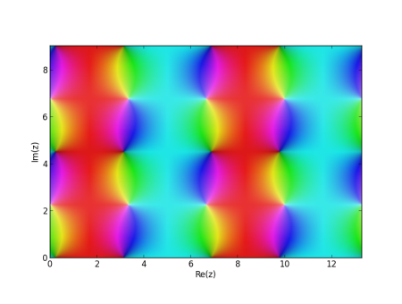
Here I’ll take a particular elliptic function sn(x). This is one of the Jacobi elliptic functions, somewhat analogous to the sine function, and use its phase portrait. Phase portraits use hue to encode the phase of a complex number, the θ value when a complex number is written in polar coordinates. The brightness of the color indicates the magnitude, the r value in polar coordinates.

Here’s the plot of sn(z, 0.2). (The sn function takes a parameter m that I arbitrarily chose as 0.2.) The plot shows two periods, horizontally and vertically. I included two periods so you could more easily see how it repeats. If you wanted to use this image as wallpaper, you could use 1/4 of the image, one period in each direction, to get by with a smaller image.

phase plot of sn(z, 0.2) - 0.2

Here’s the Python code that was used to create the image.

    from mpmath import cplot, ellipfun, ellipk
    sn = ellipfun('sn')
    m = 0.2
    x = 4*ellipk(m) # horizontal period
    y = 2*ellipk(1-m) # vertical period
    cplot(lambda z: sn(z, m) - 0.2, [0, 2*x], [0, 2*y], points = 100000)

I subtracted 0.2 from sn just to shift the color a little. Adding a positive number shifts the color toward red. Subtracting a positive number shifts the color toward blue. You could also multiply by some constant to increase or decrease the brightness.

You could also play around with other elliptic functions, described in the mpmath documentation here. And you can find more on cplot here. For example, you could supply your own function for how phase is mapped to color. The saturated colors used by default are good for mathematical visualization, but more subtle colors could be better for aesthetics.

If you make some interesting images, leave a comment with a link to your image and a description of how you made it.

Read more: Applied complex analysis

Exact chaos

Pick a number x between 0 and 1. Then repeatedly replace x with 4x(1-x). For almost all starting values of x, the result exhibits chaos. Two people could play this game with starting values very close together, and eventually their sequences will diverge.

It’s somewhat surprising that the iterative process described above can be written down in closed form. Starting from a value x0, the value after n iterations is

sin( 2n arcsin( √ x0 ) )2.

Now suppose two people start with the same initial value. One repeatedly applies 4x(1-x) and the other uses the formula above. If both carried out their calculations exactly, both would produce the same output at every step. But what if both used a computer?

The two approaches correspond to the Python functions f and g below. Because both functions are executed in finite precision arithmetic, both have errors, but they have different errors. Suppose we want to look at the difference between the two functions as we increase n.

from scipy import arcsin, sin, sqrt, linspace
from matplotlib import pyplot as plt

def f(x0, n):
    x = x0
    for _ in range(n):
        x = 4*x*(1-x)
    return x

def g(x0, n):
    return sin(2.0**n * arcsin(sqrt(x0)))**2

n = 40
x = linspace(0, 1, 100)
plt.plot(x, f(x, n) - g(x, n))
plt.ylim(-1, 1)
plt.show()

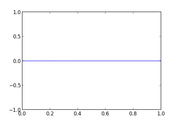
When we run the code, nothing exciting happens. The difference is a flat line.

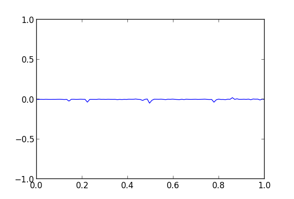
Next we increase n to 45 and we start to see the methods diverge.

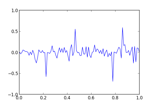
The divergence is large when n is 50.

And the two functions are nearly completely uncorrelated when n is 55.

Update

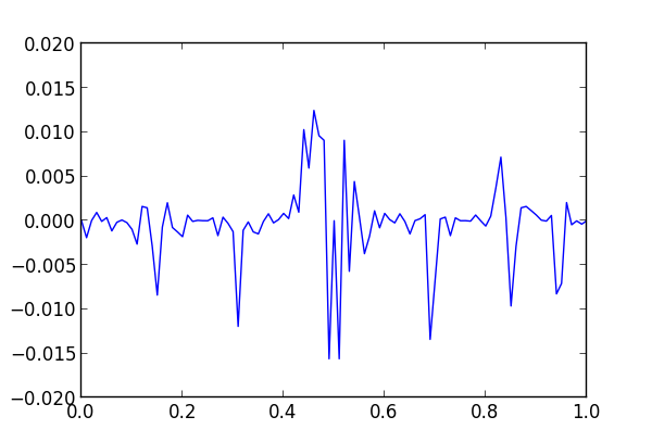
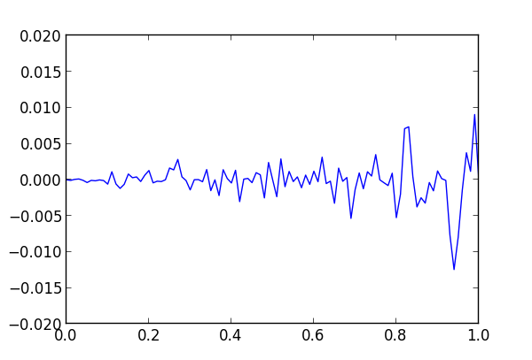
So which function is more accurate, f or g? As noted in the comments, the two functions have different kinds of numerical errors. The former accumulates arithmetic precision error at each iteration. The latter shifts noisy bits into significance by multiplying by 2^n. Apparently both about the same overall error, though they have different distributions of error.

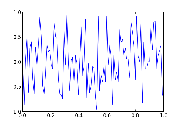
I recomputed g using 100-digit precision with mpmath and used the results as the standard to evaluate the output of f and g in ordinary precision. Here’s a plot of the errors when n = 45, first with f

and then with g.

The average absolute errors of f and g are 0.0024 and 0.0015 respectively.

Python animation for mechanical vibrations

Stéfan van der Walt wrote some Python code to animate the system described in yesterday’s post on mechanical vibrations.

Stéfan posted his code on github. It currently illustrates undamped free vibrations, but could be modified to work with damped or driven vibrations.

The code includes an option to save the output as an mp4 file. You must have ffmpeg installed to save a matplotlib animation as mp4.