If you want to add ∞ to the real numbers, should you add one infinity or two? The answer depends on context. This post gives several examples each of when its appropriate to add one or two infinities.

Two infinities: relativistic addition

A couple days ago I wrote about relativistic addition, where the sum of two numbers x and y is defined by

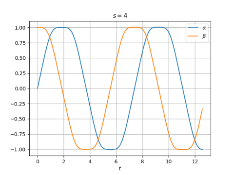
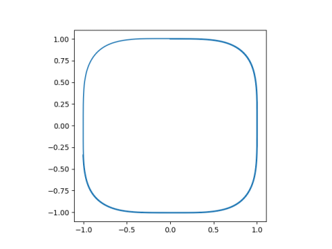
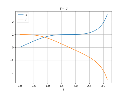
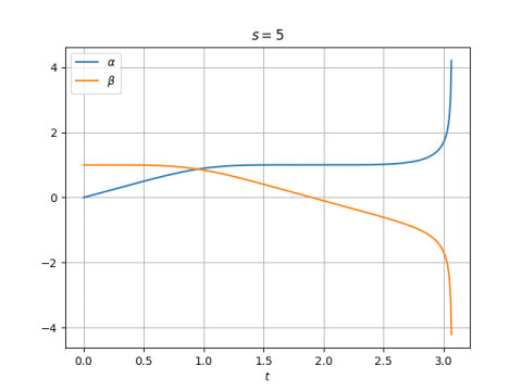
where c is some positive constant. If we restrict x and y to be inside the open interval (-c, c) there are no complications. We could extend this to the closed interval [-c, c] with c acting like ∞ and –c acting like -∞. The addition rule above is based on addition of velocities in relativity, the speed of light acting like an infinity. There are two infinities, corresponding to light traveling in opposite directions. There is one caveat: c ⊕ (-c) is undefined.

One infinity: parallel addition

Another novel way to add real numbers is parallel addition.

This kind of addition comes up often in applications. For example, the combined resistance of two resistors in parallel is the parallel sum of their individual resistances, hence the name. The harmonic mean of two numbers is twice their parallel sum.

If we understand 1/∞ to be zero, then ∞ is the identity element for parallel addition, i.e.

Now there’s only one infinity. If we incorporated -∞ it would behave exactly like ∞.

Two infinities: IEEE numbers

Standard floating point numbers have two infinities; numbers can overflow in either the positive or negative direction. For more on that, see IEEE floating point exceptions and Anatomy of a floating point number.

One infinity: Posit numbers

Posit numbers are an alternative to IEEE floating point numbers. Unlike IEEE numbers, posit numbers have only one infinity. This is graphically depicted in the unum and posit project logo below.

One advantage of posits for low-precision arithmetic because fewer bits are devoted to infinities and other exceptional numbers. The overhead of these non-numbers is relatively greater in low-precision.

For an introduction to posits, see Anatomy of a posit number.

Topology: compactification

Compactification is the process of adding points to a topological space in order to create a compact space. In topological terms, this post is about one-point compactification and two-point compactification.

The two-point compactification of the real numbers is the extended real numbers [-∞, ∞] which are homeomorphic (topologically equivalent) to a closed interval, like [0, 1].

The one-point compactification of the real numbers (-∞, ∞) ∪ ∞ is homeomorphic to a circle. Think of bending the real line into a circle with a point missing, then adding ∞ to fill in the missing point.

Parallel addition can be extended to the complex numbers, and there is still only need for one ∞ to make things complete. The one-point compactification of the complex plane is homeomorphic to a sphere.

Elliptic curves

Elliptic curves have a single point at infinity, and as with parallel addition the point at infinity is the additive identity. Interestingly, elliptic curves over finite fields have a finite number of points. That is, they have something that acts like infinity even though they do not have an infinite number of points. This shows that the algebraic and topological ideas of infinity are distinct from the idea of infinity as a cardinality.

Let c be a positive constant and define a new addition operation on numbers in the interval (-c, c) by

This addition has several interesting properties. If x and y are small relative to c, then x ⊕ y is approximately x + y. But the closer x or y get to c the more x ⊕ y differs from x + y. In fact, x ⊕ y can never escape the interval (-c, c).

The number c acts as a sort of point at infinity: c ⊕ x = c for any x in (-c, c), i.e. nothing you add to c can make it any larger.

The constant is called c after the speed of light. The addition above is simply adding x and y as velocities in special relativity.

You can show that mapping z to c tanh z gives an isomorphism from the real numbers with ordinary addition to the interval (-c, c) with ⊕ for addition. This is the transformation I used yesterday to graph a function that had too large a range to plot directly.

Update: Now that we have relativistic addition, how would we define relativistic multiplication?

William J. Milne [1] attributes the following theorem to Galileo:

The area of a circle is a mean proportional between the areas of any two similar polygons, one of which is circumscribed about the circle and the other is isoparametric with the circle.

So imagine a polygon P and let S be an inscribed circle, that is, the largest circle that can fit inside P. Also imagine a second polygon P‘ the same shape as P but with perimeter equal to that of S. Then the ratio of the area of P to the area of S equals the ratio of the area of S to the area of P‘. Said another way, the area of S is the geometric mean between the areas of P and P‘.

In the figures above, the blue pentagon is P, the black circle is S, the green pentagon is P‘, and S and P‘ have the same perimeter.

Clearly the blue pentagon has a greater area than the black circle. The isoparametric theorem says that a circle has the maximum area for a given perimeter, so the black circle must have larger area than the smaller pentagon. This doesn’t prove Galileo’s theorem, but it does prove that at least the area of the circle is somewhere in between the areas of the two pentagons.

You can prove Galileo’s theorem for regular n-gons using the formulas in this post and one other fact: the ratio of the radii of inscribed and circumscribed circles sandwiching a regular n-gon is cos(π/n).

[1] William J. Milne. Plane and Solid Geometry. 1899. p. 377, exercise 135.

The previous post looked at finding the expected number of real zeros of high degree polynomials. If you wanted to see how many real roots a particular high degree polynomial has, you run into several difficulties.

If you use something like Descartes’ rule of signs, you’re likely to greatly over-estimate the number of roots. It would be easier to plot the function and look for the roots. But this brings up a couple more problems.

First, what range should you plot over? However far out you plot, how do you know there’s not another zero outside your plot?

Second, a high-degree polynomial is likely to vary by many orders of magnitude, making it impossible to see a plot on a single scale.

The first difficulty can be overcome by a theorem of Lagrange [1] that says all the zeros of an nth degree polynomial are contained in a disk of radius

centered at the origin of the complex plane. Here a_i is the coefficient of xⁱ.

The second difficulty can be overcome by plotting a transform of the polynomial rather than the polynomial itself. The hyperbolic tangent function works well because it maps 0 to 0, and because it compresses the real line into the interval (-1, 1). It will give a distorted picture of the polynomial, but it will preserve the zeros.

We will illustrate all this with some Python code.

We can evaluate our polynomial from an array of coefficients using Horner’s method.

    def poly(coeff, x):
        p = 0.0
        for c in reversed(coeff):
            p *= x
            p += c
        return p

Next, we generate the coefficients of a random 100th degree polynomial.

    import scipy as sp
    from scipy.stats import norm
 
    sp.random.seed(20201228) # today's date

    degree = 100
    coeff = norm.rvs(size = degree+1)

Now we find Lagrange’s bounds on the roots.

    m = max(1, sum(abs(coeff[:-2]/coeff[-1])))

Now we can plot the tanh of our polynomial

    import numpy as np
    import matplotlib.pyplot as plt

    x = np.linspace(-m, m, 1000)
    y = poly(coeff, x)
    z = np.tanh(y)
    plt.plot(x, z)

This produces a plot that’s basically just a spike. Lagrange’s bound is very generous in this case, but at least we know we’ve looked widely enough to start with. if we zoom in on the spike we get the following.

If we hadn’t taken the tanh our plot would vary by over 80 orders of magnitude.

We can zoom in a bit to see the zeros more clearly.

[1] Another bound on zeros due to Cauchy is

In this example, Cauchy’s bound is tighter. You could always compute both bounds and take the smaller bound.

Suppose you create a 100th degree polynomial by picking coefficients at random from a standard normal. How many real roots would you expect?

There are 100 complex roots by the fundamental theorem of algebra, but how many would you expect to be real?

A lot fewer than I would have expected. There’s a theorem due to Kac [1] that the expected number of zeros is asymptotically

2 log(n) / π.

A higher order asymptotic series is

2 log(n) / π + 0.6257… + 2/nπ + O(n⁻²)

So for an 100th degree polynomial, you’d expect around 3 or 4 real roots.The number of roots had to be even—the only way to have an odd number of roots is with multiple roots, and such roots have   probability zero—and so four roots would be common. Of course there could be up to 100 real roots, but that is extremely unlikely.

It turns out a polynomial would have to have degree over two million before the expected number of roots would 10.

Related posts

• Descartes and toolz
• Plotting roots of a high-degree polynomial
• Random polynomials revisited

[1] Alan Edelman and Eric Kostlan. How many zeros of a random polynomial are real? Bulletin of the AMS. Volume 32, Number 1, January 1995