Differential Equations and Department Stores

Posted on 30 August 2021 by John

Howard Aiken on the uses of computers, 1955:

If it should turn out that the basic logics of a machine designed for the numerical solution of differential equations coincide with the basic logics of a machine intended to make bills for a department store, I would regard this as the most amazing coincidence I have ever encountered.

Update: Some people have read the quote above and thought Aiken was ignorant of the work of Turing et al. I assumed he was speaking in terms of what was practical rather than what was possible, which is apparently correct.

Thanks to Anatoly Vorobey in the comments below, I found a paper that goes into more background. From that paper:

Aiken’s theme in the lecture … was that a machine designed primarily for scientific use was far from ideal for business computing. … For example, scientific computing (Aiken pointed out) involves relatively small amounts of data and complex processing, whereas business computing involves large amounts of data and relatively shallow processing.

Empirical formula for the shape of an egg

Posted on 28 August 2021 by John

A while back I wrote about a simple equation for the shape of an egg. That equation is useful for producing egg-like images, but it’s not based on extensive research into actual eggs.

I recently ran across a more realistic, but also more complicated, equation for modeling the shape of real eggs [1]. The equation models the shape of an egg by rotating the graph of a function of the form

y = (B/2) f(x; L, w, D)

around the x-axis. The parameters B and L are simple to describe, but w and D take a little more explanation.

Parameters

Imagine the egg positioned so the x-axis runs along the center of the egg, with the fat end on the left at −L/2 and the pointy end on the right at L/2. So L is the length of the egg.

The parameter B is the maximum breadth of the egg, the maximum diameter perpendicular to the central axis. If you plot y above as a function of x, the maximum value of y is B/2.

The authors describe w as “the parameter that shows the distance between two vertical axes corresponding to the maximum breadth and the half length of the egg.” I find that description confusing. I believe they’re saying that −w is the location of the maximum of y. So B/2 is the maximum value of y, and –w is where that maximum occurs.

The authors define a parameter D_L/4 that I’m calling D for simplicity. They define this parameter as the “egg diameter at the point of L/4 from the pointed end.” That is, D is twice the value of y at x = L/4. Recall that the egg runs from −L/2 to L/2, so we’re talking about the point 3/4 of the way between the fat end and the pointed end.

To summarize, L, B, w, and D are the length, maximum breadth, the negative of the location of the maximum breadth, and the breadth three quarters of the way between the fat and pointed ends.

Equation

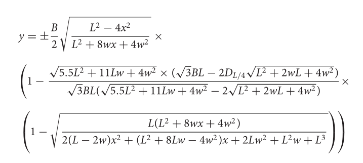
With all that out of the way, here’s the equation. I’ll write it up in Python, but I wanted to include a screen shot from the paper in case I made an error in coding it up.

sorry, it's complicated

Python implementation

Here’s Python code that implements this function, if I haven’t made any errors.

    from numpy import sqrt

    def egg_radius(x, L, B, w, D):

        # Note that k does not involve x
        k = sqrt(5.5*L**2 + 11*L*w + 4*w**2)
        k *= sqrt(3)*B*L - 2*D*sqrt(L**2 + 2*w*L + 4*w**2)
        k /= sqrt(3)*B*L
        k /= sqrt(5.5*L**2 + 11*L*w + 4*w*w) - 2*sqrt(L**2 + 2*w*L + 4*w**2)

        # coefficients of a quadratic in x
        a = 2*(L-2*w)
        b = L**2 + 8*L*w - 4*w**2
        c = 2*L*w**2 + L**2*w + L**3
    
        t = L*(L**2 + 8*w*x + 4*w**2)
        t /= a*x**2 + b*x + c

        y = 0.5*B*sqrt(L**2 - 4*x**2)/sqrt(L**2 + 8*w*x + 4*w**2)    
        y *= (1 - k*(1 - sqrt(t)))

        return y

Here’s a plot using this code:

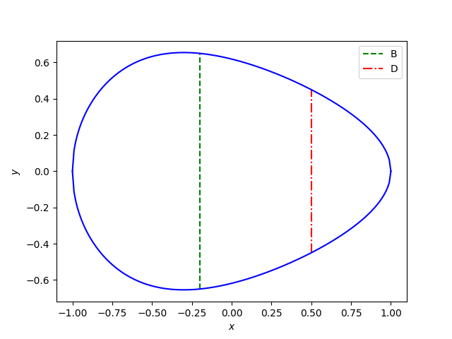
And here’s the code that was used to make the plot:

    from numpy import linspace
    import matplotlib.pyplot as plt

    L = 2
    B = 1.3
    w = 0.2
    D = 0.9

    plt.plot([-w, -w], [-B/2, B/2], 'g--')
    z = egg_radius(L/4, L, B, w, D)
    plt.plot([L/4, L/4], [-z, z], "r-.")
    x = linspace(-L/2, L/2, 200)
    y = egg_radius(x, L, B, w, D)
    plt.plot(x, y, 'b')
    plt.plot(x, -y, 'b')
    plt.legend(["B", "D"])
    plt.xlabel("$x$")
    plt.ylabel("$y$")
    plt.show()

Error

Something does add up. It appears that y(−w) = B, as it should, but the maximum of y is not at −w.

    from scipy.optimize import minimize_scalar

    print(-w, egg_radius(-w, L, B, w, D))
    res = minimize_scalar(lambda x: -egg_radius(x, L, B, w, D), bracket=[-1,0,1], method='brent')
    print(res.x, egg_radius(res.x, L, B, w, D))

This shows the maximum is near −0.3, not at −0.2.

Maybe I’ve misunderstood something or made a coding error. Or maybe there’s an error in the paper.

Maybe the breadth you specify is a target and not something that is always exactly achieved?

***

[1] Egg and math: introducing a universal formula for egg shape. Valeriy G. Narushin, Michael N. Romanov, Darren K. Griffin. Annals of the New York Academy of Sciences. Published online August 23, 2021.

Computing ζ(3)

Posted on 28 August 2021 by John

I’ve started reading Paul Nahin’s new book “In Pursuit of ζ(3).” The actual title is “In Pursuit of Zeta-3.” I can understand why a publisher would go with such a title, but I assume most people who read this blog are not afraid of Greek letters.

I’ve enjoyed reading several of Nahin’s books, so I was pleased to see he had a new one.

Nahin’s latest book is about attempts to find a closed-form expression for the sum

$\sum_{n=1}^\infty \frac{1}{n^3}$

If you replace the “3” with “s” in the sum above, you have an expression for the Riemann zeta function ζ(s), and so ζ(3) is a convenient way of describing the sum and putting it in context [1]. There are closed-form expressions for ζ(s) when s is an even integer [2] but so far not nobody has found one for s = 3.

The value of ζ(3) is sometimes called Apéry’s constant because in 1978 Roger Apéry was the first to prove that it is an irrational number.

The names “ζ(3)” and “Apéry’s constant” are anachronisms because Euler studied the sum in the 18th century, but Riemann came along in the 19th century and Apéry in the 20th.

Naive calculation

The most obvious way to compute ζ(3) numerically is to replace the upper limit of the infinite sum with a large number N. This works, but it’s very inefficient.

Let’s calculate the sum with upper limit 100 with a little Python code.

    >>> sum(n**-3 for n in range(1, 101))
    1.2020074006596781

We can judge the accuracy of this approximation using the implementation of the zeta function in SciPy.

    >>> from scipy.special import zeta
    >>> zeta(3)
    1.2020569031595942

We can predict how accurate our sum will be by estimating the tail of the sum using the integral test as follows.

$\int_{N}^\infty x^{-3} \, dx >\sum_{n = N+1}^\infty n^{-3} > \int_{N+1}^\infty x^{-3} \, dx$

The integral on the left evaluates to N⁻²/2 and the integral on the right evaluates to (N + 1)⁻²/2.

This says that if we sum up to N, our error will be between (N + 1)⁻²/2 and N⁻²/2.

We can estimate from this that if we want d decimal places, we’ll need to sum 10^d/2 terms. So to get 16 decimal places, we’d have to sum 100,000,000 terms. This is certainly not what the call to zeta(3) above is doing.

A better approach

Nahin’s book derives an equation for ζ(3) by Ernst Kummer (1810–1893):

$\zeta(3) = \frac{5}{4} - \sum_{n=2}^\infty \frac{1}{n^3(n^2-1)}$

Because the denominator in the sum is a 5th degree polynomial, we get faster convergence than we do from directly evaluating the definition of ζ(3). We could find an interval around the error using the integral test above, and it would show that the error is O(N⁻⁴).

Let’s try this out in Python.

    >>> f = lambda n: (n**3 * (n**2-1))**-1
    >>> 1.25 - sum(f(n) for n in range(2, 101))
    1.2020569056101726
    >>> _ - zeta(3)
    2.4505784068651337e-09

This says we get 8 correct decimal places from summing 100 terms, which is just what we’d expect from our error estimate.

Doing even better

Kummer’s approach is better than naively computing ζ(3) from its definition, but there are much more efficient methods.

With naive summation up to N, we get

2 log₁₀ N

correct decimals. With Kummer’s sum we get twice as many,

4 log₁₀ N

correct decimals.

But there are methods for which the number of correct decimals is linear in N rather than logarithmic. Wikipedia mentions a method that gives 5.04 N decimal places.

Update: See this post for a sequence of more efficient algorithms.

[1] That’s how the Riemann zeta function is defined for s with real part greater than 1. For the rest of the complex plane, except s = 1, the Riemann zeta function is defined by analytic continuation. The sum is not valid for s with real part less than 1, and so, for example, the sum makes no sense at s = −1. But the analytic continuation of the sum is valid at −1, and equals −1/12 there. This leads to the rigorous justification of the otherwise nonsensical expression

1 + 2 + 3 + … = −1/12.

[2] For s = 2n where n is a positive integer,

$\zeta(2n) = \frac{(-1)^{n+1}B_{2n}(2\pi)^{2n}}{2(2n)!}$

For s = 0 and negative integers, we have

$\zeta(-n)= (-1)^n\frac{B_{n+1}}{n+1}$

Here the B‘s are the Bernoulli numbers, which have closed-form expressions.

Encryption in groups of unknown order

Posted on 25 August 2021 by John

One way of looking at RSA encryption, a way that generalizes to new methods, is that the method is based on group operations inside a group of unknown order, i.e. unknown to most people. Another way of putting it is that RSA encryption takes place in a group where everybody knows how to multiply but not everyone knows how to divide. This will be explained below.

RSA encryption starts by finding two large primes p and q. You compute the product

n = pq

and make it public, but keep the factors p and q secret. The RSA method lets anyone send you encrypted messages by doing certain operations in the multiplicative group of the integers mod n. (Details here.) Let’s call this group G.

The elements of G are the integers from 1 to n − 1 that are relative prime to n. The group operation is multiplication mod n, i.e. to multiply two elements of G, multiply them first as ordinary integers, then divide the result by n and keep the remainder.

The order of G, the number of elements in G, is

φ(n) = (p − 1)(q − 1).

You know p and q, and so you know φ(n), but the public does not. The security of RSA depends on the assumption that the public cannot compute φ(n). If someone could factor n, they could compute φ(n), but it is assumed that for large enough p and q it is not computationally feasible to factor n.

The public knows how to multiply in G but not how to divide. That is, anyone can carry out multiplication, but they cannot compute multiplicative inverses. Only you know how to divide in G, because you know φ(n) and Euler’s theorem.

In some sense the public knows everything there is to know about G. It’s the multiplicative group of integers mod n, and you tell them what n is. And that does tell them all they need to know to send you messages, but in practice it doesn’t tell them enough to decrypt messages anyone else sends you.

When you’re using RSA for public key cryptography, you’re telling the world “Here’s an n. To communicate securely with me, carry out certain algorithms with the integers relatively prime to n.”

Someone might object “But how do we know whether an integer is relatively prime to n? You haven’t told us its factors.”

You could reply “Don’t worry about it. It’s extremely unlikely that you’d run into a number that isn’t relatively prime to n. In fact, if you did, you’d break my system wide open. But if you’re worried about it, you can efficiently confirm that your numbers are relatively prime to n.”

Let’s unpack that last statement. We’ve already said that the number of positive integers less and n and relatively prime to n is (p – 1)(q – 1). So the number that are not relatively prime is

pq − (p − 1)(q – 1) = p + q − 1

and the probability of accidentally running into a one of these numbers is

(p + q − 1)/pq

Now if p and q are 300 digit numbers, for example, then this probability is on the order of one chance in 10³⁰⁰.

The Euclidean algorithm lets you find the greatest common factor of enormous numbers quickly. If you have a number k and you want to test whether it’s relatively prime to n, you can compute gcd(k, n). If k was chosen at random, the gcd is extremely likely to be 1, i.e. relatively prime to n. But if the answer is not 1, then it’s either p or q, in which case you’ve broken the encryption.

***

If you can factor large numbers, you can break RSA encryption. But it’s conceivable that you may be able to break RSA without being able to factor large numbers. That is in fact the case when RSA is implemented poorly. But aside from implementation flaws, nobody knows whether breaking RSA is as hard as factoring. Michael Rabin came up with a variation on RSA that is provably as hard as factoring, though I don’t know whether it has ever been used in practice.

Logic in moral terminology

Posted on 24 August 2021 by John

I got an email from Fr. John Rickert today, and with his permission I’ll share part of it here.

A sin of commission occurs when we do something we should not do. A system is consistent (or maybe I should say “sound”) if the results of proofs really are true. Gödel’s 2nd Incompleteness Theorem says that it is undecidable whether Peano Arithmetic commits any “sins of commission.”

A sin of omission occurs when we fail to do something that we should do. A system is complete if every true statement actually has a proof (in finitely many steps). Gödel’s 1st Incompleteness Theorem says that Peano Arithmetic does commit some “sins of omission”: There are truths that cannot be proved.

Finally, a conscience is perplexed if it does not know whether to do or refrain from a proposed action; the conscience is de facto in a state of invincible ignorance. Undecidability is invincible ignorance.

Of course a formal system isn’t under any moral obligations, and certainly not under obligation to do what it cannot do. These are just analogies. But they are interesting analogies. Sins of commission and omission, things done and things left undone, are more verbally parallel than completeness and soundness.

Here’s another post based on an email exchange with Fr. Rickert exactly one year ago: Unexpected square wave.

Missing data

Posted on 24 August 2021 by John

Missing data throws a monkey wrench into otherwise elegant plans. Yesterday’s post on genetic sequence data illustrates this point. DNA sequences consist of four bases, but we need to make provision for storing a fifth value for unknowns. If you know there’s a base in a particular position, but you don’t know what its value is, it’s important to record this unknown value to avoid throwing off the alignment of the sequence.

There are endless debates over how to handle missing data because missing data is a dilemma to be managed rather than a problem to be solved. (See Problems vs Dilemmas.)

It’s simply a fact of life that data will be incomplete. The debate stems from how to represent and handle missingness. Maybe the lowest level of a software application represents missing data and the highest uses complete data only. At what level are the missing values removed and how they are removed depends very much on context.

A naive approach to missing data is to not allow it. We’ve all used software that demands that we enter a value for some field whether a value exists or not. Maybe you have to enter a middle name, even though you don’t have a middle name. Or maybe you have to enter your grandfather’s name even though you don’t know his name.

Note that the two examples above illustrate two kinds of missing data: one kind does not exist, while the other certainly exists but is unknown. In practice there are entire taxonomies of missing data. Is in unknown or non-existent? If it is unknown, why is it unknown? If it does not exist, why doesn’t it?

There can be information in missing information. For example, suppose a clinical trial tracks how long people survive after a given treatment. You won’t have complete data until everyone in the study has died. In the mean time, their date of death is missing. If someone’s date of death is missing because they’re still alive, that’s information: you know they’ve survived at least until the current point in time. If someone’s date of death is missing because they were lost to followup, i.e. they dropped out of the study and you lost contact with them, that’s different.

The simplest approach to missing data is throw it away. That can be acceptable in some circumstances, particularly if the amount of missing data is small. But simply discarding missing data can be disastrous. In wide data, data with many different fields per subject, maybe none of your data is complete. Maybe there are many columns and every row is missing something in at least one column.

Throwing away incomplete data can be inefficient or misleading. In the survival study example above, throwing out missing data would give you a very pessimistic assessment of the treatment. The people who lived the longest would be excluded precisely because they’re still living! Your analysis would be based only on those who died shortly after treatment.

Analysis of data with missing values is a world unto itself. It seems paradoxical at first to devise ways to squeeze information out of data that isn’t there. But there are many ways to do just that, each with pros and cons. There are subtle ways to infer the missing values, while also accounting for the fact that these values have been inferred. If done poorly, this can increase bias, but if done well it decreases bias.

Analysis techniques that account for missing data are more complicated than techniques that do not. But they are worth the effort if throwing away missing data would leave you with too little data or give you misleading results. If you’re not concerned about the former, perhaps you should be concerned about the latter. The bias introduced by discarding incomplete data could be hard to foresee until you’ve analyzed the data properly accounting for missing values.

Also a crypto library

Posted on 23 August 2021 by John

The home page for the OpenSSL project says

OpenSSL is a robust, commercial-grade, and full-featured toolkit for the Transport Layer Security (TLS) and Secure Sockets Layer (SSL) protocols. It is also a general-purpose cryptography library. …

If you’ve never heard of the project before, you would rightly suppose that OpenSSL implements SSL (and its successor TLS). But you might not realize that OpenSSL “is also a general-purpose cryptography library.”

After thinking about it a bit, you might realize that software implementing SSL must have some encryption capability, but it doesn’t follow that this capability would necessarily be readily accessible. In fact, OpenSSL has implements a lot of cryptography algorithms and makes them easy to use from the command line. For example, this post shows how to compute hash functions using the openssl command.

Earlier today I wrote a thread on @CompSciFact about the famous example of encrypting an image of the Linux mascot Tux using ECB (Electronic Code Book) mode. As the saying goes, you should never use ECB “because you can see the penguin.”

Original encrypted Tux image

I wanted to try reproducing the example, and my first thought was to use Python. But setting up encryption libraries is a fairly lengthy process, while AES encryption using openssl is a one-liner.

My encrypted Tux image

You can still see the outline of Tux, but my penguin looks quite different from the famous example for a variety of reasons. For starters, I don’t know what key was used in the original image. Also, there are a variety of ways to extract the data from an image, encrypt it, and put it back. I basically followed Filippo Valsorda’s post The ECB Penguin but I had to make a few changes to get it to work due to changes in GIMP since that post was written.

Naive compression of genetic data

Posted on 23 August 2021 by John

There are special compression algorithms for genetic sequence data, but I was curious how well simply zipping a text file would work.

I downloaded a 14 MB text file containing DNA sequence data from a fruit fly and compressed it as a zip file and as a 7z file. The result was about 3.5 MB, which is basically no compression beyond the obvious.

The file contains millions of A’s, C’s, G’s, and T’s and nothing more [0]. (I prepared the file by removing comments and line breaks.)

    AAAATCAATATGTTGCCATT…

There are only four possible characters, so each carries two bits of information [1], but is encoded in an 8-bit ASCII character. The most obvious encoding would pack four letters into a byte. That would compress a 14 MB text file down to a 3.5 MB binary file.

Here are the exact numbers.

|----------+----------+-------|
| file     |     size |  ratio|
|----------+----------+-------|
| original | 14401122 | 1.000 |
| zip      |  3875361 | 3.716 |
| 7z       |  3419294 | 4.212 |
|----------+----------+-------|

So the 7z format does a little better than simply packing groups of four letters into a byte, but the zip format does not.

There is repetition in genome sequences, but apparently generic compression software is unable to exploit this repetition. You can do much better with compression algorithms designed for genetic data.

Update

The plot thickens. Imran Haque kindly let me know that I overlooked the N’s in the data. These are placeholders for unresolved bases. You can’t simply encode each base using two bits because you need five states.

The number of N’s is small—at least in this example, though I imagine they would be more common in lower quality data—and so the calculation in footnote [1] is still approximately correct [2]. There are about two bits of information in each base, but this is on average. Shannon would say you can expect to compress your text file by at least 75%. But you can’t simply represent each base with two bits as I suggested because you need to make room for the possibility of a null base.

Note that the total information of a file is not the number of symbols times the information per symbol, unless all the symbols are independent. In the case of genetic data, the symbols are not independent, and so more compression is possible.

***

[0] Or so I thought. See the Update section.

[1] The letter frequencies are not exactly equal, but close: 26.75% A, 23.67% C, 23.94% G, and 25.58% T. The Shannon entropy is 1.998, so essentially two bits.

[2] N’s account for 0.04% of the data. Accounting for the N’s increases the Shannon entropy to 2.002.

FM signal approximation

Posted on 22 August 2021 by John

FM radio transmits a signal by perturbing (modulating) the frequency of a carrier wave. If the carrier has frequency ω and the signal has frequency q, then the FM signal is

cos(ωt + β cos(qt)).

To understand the modulated signal, it’s useful to write it as a sum of simple sines and cosines with no modulation. I wrote about how to do this exactly using Bessel functions. Today I’ll write about an approximation that’s easier to understand and work with, assuming the modulation index β is small.

Here’s the approximation:

cos(ωt + β cos(qt)) ≈ cos ωt + ½ β ( sin (ω + q)t + sin (ω − q)t ).

This says that to a good approximation, the modulation term adds two sine waves to the carrier, one that adds the signal frequency to the carrier frequency and one that subtracts it.

To establish the approximation and see how the error depends on β, subtract the right side from the left and expand as a Taylor series in β. The first non-zero term in the series is

-½ cos(qt)² cos(ωt) β²

and so if β is small, the approximation error is very small. For example, if β = 0.1, then the approximation error is on the order of 0.005.

As an example, let ω = 10, q = 2, and β = 0.1. Then

cos(10t + 0.1 cos 2t) ≈ cos 10t + 0.05 ( sin 12t + sin 8t )

and the approximation error is plotted below.

As predicted, the amplitude of the error is around 0.005, while the amplitude of the FM signal is 1.

Month: August 2021