Three interesting curves

Posted on 6 November 2022 by John

Here are three curves that have interesting names and interesting shapes.

The fish curve

The fish curve has parameterization

x(t) = cos(t) – sin²(t)/√2
y(t) = cos(t) sin(t)

We can plot this curve in Mathematica with

    ParametricPlot[
        {Cos[t] - Sin[t]^2/Sqrt[2], Cos[t] Sin[t]}, 
        {t, 0, 2 Pi}]

to get the following.

Fish curve

It’s interesting that the image has two sharp cusps: the parameterization consists of two smooth functions, but the resulting image is not smooth. That’s because the velocity of the curve is zero at 3π/4 and 7π/4.

I found the fish curve by poking around Mathematica’s PlainCurveData function. I found the next two in the book Mathematical Models by H. Martyn Cundy and A. P. Rollett.

The electric motor curve

Next is the “electric motor” curve. Cundy and Rollett’s book doesn’t provide illustrations for the plane curves it lists on pages 71 and 72, and I plotted the electric motor curve because I was curious why it was called that.

The curve has equation

y²(y² − 96) = x² (x² − 100)

and we can plot it in Mathematica with

    ContourPlot[ y^2 (y^2 - 96) == x^2 (x^2 - 100), 
        {x, -20, 20}, {y, -20, 20}

which gives the following.

electric motor curve

Sure enough, it looks like the inside of an electric motor!

The ampersand curve

I was also curious about the “ampersand curve” because of its name. The curve has equation

(y² − x²) (x − 1) (2x − 3) = 4 (x² + y² − 2x)²

and can be plotted in Mathematica with

    ContourPlot[(y^2 - x^2) (x - 1) (2 x - 3) == 
                 4 (x^2 + y^2 - 2 x)^2, 
                 {x, -0.5, 2}, {y, -1.5, 1.5}, 
                 PlotPoints -> 100]

The produces the following pleasant image.

ampersand curve, smooth version

Note that the code specifies PlotPoints. Without this argument, the default plotting resolution produces a misleading plot, making it appear that the curve has three components.

Ampersand curve, misleading version plotted with too few points

What is a Pentanomial GFSR random number generator?

Posted on 6 November 2022 by John

The ISO random number generation standard, ISO 28640, speaks of a “Pentanomial GFSR method” for generating random variates. What is this? We’ll break it down, starting with GFSR.

GFSR

In short, a GFSR random number generator is what is now more commonly called a linear feedback shift register, or LFSR. The terminology “GFSR” was already dated when the ISO standard was published in 2010.

Tausworthe [1] came up with LFSR random variate generators in 1965. His paper looked at linear feedback shift registers but doesn’t use the term LFSR. LFSRs are bit sequences in which the current bit is a linear combination of certain previous bits, something like a Fibonacci sequence. The algebra is being carried out mod 2, so addition amounts to XOR.

As a toy example, consider

x_n+5 = x_n+2 + x_n.

The first five bits would be the seed for the generator, then the recurrence above determines the rest. So, for example, we might start with 01101. Then the sequence of bits would be

011011101010000100101100111110001101110101…

It seems the term GFSR dates to 1973 with Lewis and Payne [2]. As far as I can tell, between 1965 and 1973 Tausworthe’s idea was implemented in practice using two previous terms, and this specialization of LFSRs became known as FSRs. Then [2] generalized this to include possibly more previous terms, restoring the generality of [1].

That explains “GFSR method” but what is this “pentanomial”?

Pentanomial

Recurrence relations can be described in terms of their characteristic polynomials. For example, in the familiar Fibonacci sequence

F_n+2 = F_n+1 + F_n

the characteristic polynomial is

x² − x − 1.

The characteristic polynomial of the toy generator above would be

x⁵ − x² − 1.

And since −1 is the same as 1 when working mod 2, we’d usually write this polynomial as

x⁵ + x² + 1.

Between 1965 and 1973 FSRs were implemented by terms that had a trinomial as the characteristic polynomial. Lewis and Payne looked at recurrences that depended on more previous terms, and in particular the choice of 4 previous terms, corresponding to a polynomial with 5 non-zero coefficients, had nice properties, hence the term “pentanomial.”

Primitive polynomials

The polynomials come before the recurrences. That is, we don’t write down the polynomial after designing the recurrence; the recurrence is designed by picking characteristic polynomials with special algebraic properties. This is because a primitive polynomial corresponds to the longest possible sequence of bits before things repeat.

The period of a LFSR corresponding to an nth degree primitive polynomial is 2ⁿ-1. This is the maximum possible because we cannot seed an LFSR with all zeros. We could, but the sequence would only produce zeros. As long as at least one bit in the seed is set, the LFSR will produce a sequence of 2ⁿ-1 bits before repeating.

Practicalities

In practice LFSRs are based on higher-degree polynomials than our toy example. For example, one might use

x_n+607 = x_n + x_n+167 + x_n+307 + x_n+461

after seeding it with 607 random bits. This corresponds to the primitive pentanomial

x⁶⁰⁷ + x⁴⁶¹ + x³⁰⁷ + x¹⁶⁷ + 1.

This LFSR would have period 2⁶⁰⁷ − 1, or on the order of 10¹⁸³ bits.

LFSRs are very fast, but they’re unsuitable for cryptography because linear feedback is linear and cryptanalysis can exploit linear structure. So in order to use LFSRs as secure random number generators they have to be combined with some sort of nonlinear processing, such as described here.

Systematically solving trigonometric equations

Posted on 5 November 2022 by John

Students are asked to solve trigonometric equations shortly after learning what sine and cosine are. By some combination of persistence and luck they may be able to find a solution. After proudly presenting the solution to a teacher, the teacher may ask “Is that the only solution?” A candid student would respond by saying “How should I know?!”. The omniscient teacher, having seen the solution, declares that there is another.

Trigonometric equations pop up fairly often in applications, but thoroughly solving such equations requires algebraic techniques that are not typically part of the undergraduate curriculum.

This post will present a terse outline of a systematic way to approach trigonometric equations that are polynomials in sines and cosines of integer multiples of an angle θ.

First, get rid of all the multiples of θ by using multiple angle identities.

$\begin{align*} \cos(n\theta) &= 2 \cos(\theta) \cos((n-1)\theta) - \cos((n-2)\theta) \\ \sin(n\theta) &= 2 \cos(\theta) \sin(\,(n-1)\theta) - \sin(\,(n-2)\theta) \end{align*}$

By repeatedly applying these identities we can reduce terms involving integer multiples of θ to terms involving only sums and products of sin(θ) and cos(θ).

Next, given a trigonometric equation of the form

$P(\sin\theta, \cos\theta) = 0$

where P is a polynomial in two variables, we turn it into a system of two polynomial equations

$\begin{align*} P(s, c) &= 0 \\ s^2 + c^2 - 1 &= 0 \end{align*}$

by introducing s = sin(θ) and c = cos(θ).

Now we have a purely algebraic system of two polynomials in two variables. A system of two polynomials in one variable have a common solution if and only if their resultant is zero. We can think of a polynomial in two variables as a polynomial in one variable whose coefficients are polynomials in the other variable.

If we think of our polynomial in s and c as a polynomials s with coefficients given by polynomials in c, then the condition that the resultant equals zero gives a polynomial equation in c that solutions must satisfy.

In short, we reduce a trigonometric equation to a system of two polynomial equations in two unknowns, and then to a single polynomial equation in one unknown. In general the final polynomial will have high degree, and so finding its roots will take some work, but it’s a routine problem.

Nephroids and evolutes

Posted on 4 November 2022 by John

The previous post looked at the evolute of an ellipse. This post will look at evolutes more generally, and then look at nephroids.

As a quick reminder, given a curve c, a point on its evolute is the center of curvature for a point on c. See the previous post for a detailed example.

If a curve has a parameterization (x(t), y(t))^T then its evolute has parameterization

$\begin{pmatrix}x(t) \\ y(t) \end{pmatrix} - \frac{x'(t)^2+y'(t)^2}{x'(t) y''(t)-x''(t) -y'(t)} \begin{pmatrix}y'(t) \\ x'(t) \end{pmatrix}$

Nephroid curve

Let’s apply this to a nephroid. This word comes from the Greek for kidney-shaped. Comes from the same root as nephrology.

A nephroid can be parameterized by

$\begin{pmatrix} 3\cos t - \cos 3t \\ 3\sin t - \sin 3t \end{pmatrix}$

When we compute the evolute for this curve we get

$\begin{pmatrix} 2\cos^3 t \\ (2 + \cos 2t)\sin t \end{pmatrix}$

It’s not apparent from the expression above that the evolute of an nephroid is another nephroid, but it is clear from the plot below.

The solid blue curve is the nephroid, and the dashed orange curve is its evolute. Apparently the evolute is another nephroid, rotated and rescaled. We’ll come back to the equations shortly, but let’s look at another example first.

Cayley’s sextit

There is a curve known as Cayley’s sextit that has parameterization

$\begin{pmatrix} \cos^3 (t/3) \,\cos (t) \\ \cos^3 (t/3) \,\sin (t) \end{pmatrix}$

When we compute the evolute of this curve we get

$\begin{pmatrix} -\cos^2(t/3) (-2 \cos(2t/3) + \cos(4t/3)) / 2 \\ \sin^3(2t/3)/4 \end{pmatrix}$

When we plot Cayley’s sextit and its evolute we get

Note that to get the full curve of the evolute we let t run from 0 to 4π.

Again it’s not at all obvious from the equations, but apparently the evolute of Cayley’s sextit is also a nephroid, this time scaled, stretched, and shifted.

This says that pre-evolutes are not unique: two different curves can have the same (family) of evolutes.

Algebra

Now for the hard part: doing the algebra to show that the curves that look like nephroids are indeed nephroids.

We need to show that the set of points traced out by the evolute is a set of points on a nephroid: we don’t have to show that our parameterization of the evolute can be turned into our parameterization of a nephroid. So we shift to an implicit equation for a nephroid, scaled by a factor a:

$((x^2 + y^2 - 4a^2)^3 = 180 \,a^4 y^2$

Nephroid evolute

First let’s show that the evolute of a nephroid is a nephroid. From the plot it appears that the evolute is scaled by 1/2 and rotated a quarter turn. So we suspect that if we reverse x and y and multiply both by 1/2 we’ll get a nephroid. Let’s let Mathematica verify this for us:

    implicit[x_, y_, a_] := (x^2 + y^2 - 4 a^2)^3 - 108 a^4 y^2
    Simplify[implicit[(2 + Cos[2 t]) Sin[t], 2 Cos[t]^3, 1/2]]

Without calling Simplify we get something that isn’t obviously zero, but applying trig identities can reduce it to zero.

Cayley’s sextit evolute

In order to show that the evolute of Cayley’s sextit is a nephroid, we have to find what nephroid we believe it is.

Let’s look at the our parameterization of a nephroid again:

$\begin{pmatrix} 3\cos t - \cos 3t \\ 3\sin t - \sin 3t \end{pmatrix}$

We can see that the two cusps are at (-2, 0) and (2, 0), and the minimum and maximum heights are (0, -4) and (0, 4). We’ll line these points up with their counterparts in the evolute to Cayley’s sextit. Let’s look at its parameterization.

$\begin{pmatrix} -\cos^2(t/3) (-2 \cos(2t/3) + \cos(4t/3)) / 2 \\ \sin^3(2t/3)/4 \end{pmatrix}$

The two cusps correspond to y = 0, which happens when t = 0 and t = 3π/2. The corresponding x values are 1/2 and 0. This suggests the center of our nephroid is at 1/4 and our nephroid has been scaled by 1/8 in the horizontal direction.

The top and bottom correspond to x = 1/4, which happens when t = 3π/4 and t = 9π/4, and so our nephroid has height 1/4. This says our nephroid has been scaled by 1/16 in the vertical direction.

So if we shift x by 1/4 then multiply by 8, and multiply y by 16, we suspect we’ll get a standard nephroid. Let’s see what Mathematica has to say.

    implicit[8(-Cos[t/3]^2 (-2 Cos[2 t/3] + Cos[4 t/3])/2 - 1/4), 
        16 Sin[2 t/3]^3/4, 1]

This confirms that our guesses were correct. The evolute of Cayley’s sextit is indeed a nephroid, and we’ve identified which nephroid it is.

Evolute of an ellipse

Posted on 4 November 2022 by John

Suppose you’re standing on an ellipse. (You actually are: lines of longitude are elliptical because of earth’s equatorial bulge.)

Now draw a line perpendicular to where you’re standing. Lines of longitude are nearly circles, but we’ll look at a more obviously elliptical ellipse.

ellipse with one normal line

The line is perpendicular to the northeast side of the ellipse where it starts, but not where it crosses on the other side.

Now suppose lots of people standing on the circle all draw perpendicular lines. We get a surprising result.

If we did this with a circle, all we’d see is lines radiating out of the center of the circle. But for an ellipse we get something much more interesting.

There’s a simple equation for the star-like figure in the middle created by all the normal lines. We’ll get to that shortly, but first we need to talk about kissing circles.

Kissing circles

Suppose you wanted to approximate an ellipse by pieces of a circle, as is sometimes done in computer graphics. What radius should you use?

The circle that best approximates a curve at a point is called the kissing circle, or classically the osculating circle. The radius of this circle is the radius of curvature at the point where it touches the curve.

ellipse with two kissing circles

In the image above, the small blue circle is the best approximation of the ellipse on the side. The much bigger green circle is the best approximation to the ellipse on the top. The centers of these two circles are the centers of curvature at the two points on the curve.

Equation of evolute

We could visualize all centers of curvature by plotting the center of curvature for each point on the curve. This is called the evolute of the curve.

If we parameterize our ellipse by

x(t) = a cos t
y(t) = b sin t

then the evolute has parameterization

x(t) = (a² − b²) cos³ t / a
y(t) = (b² − a²) sin³ t / b

You can find a general formula for the evolute to any parameterized curve in the next post.

Here’s what it looks like.

This is the same shape as the figure formed by the normal lines at the top of the post. The lines that are normal to the ellipse are tangent to its evolute. To confirm this, we’ll plot the normal lines again and plot the evolute on top in red.

Incidentally, the evolute of an ellipse can extend outside the ellipse, and it will if the ellipse is more eccentric. Here’s an example.

The next post looks at a curve whose evolute is another curve of the same kind.

Newton’s method: The Good, The Bad, and The Ugly

Posted on 3 November 2022 by John

This post will give examples where Newton’s method gives good results, bad results, and really bad results.

Our example problem is to solve Kepler’s equation

M = E − e sin E

for E, given M and e, assuming 0 ≤ M ≤ π and 0 < e < 1. We will apply Newton’s method using E = M as our starting point.

The Good

A couple days ago I wrote about solving this problem with Newton’s method. That post showed that for e < 0.5 we can guarantee that Newton’s method will converge for any M, starting with the initial guess E = M.

Not only does it converge, but it converges monotonically: each iteration brings you closer to the exact result, and typically the number of correct decimal places doubles at each step.

You can extend this good behavior for larger values of e by choosing a better initial guess for E, such as Machin’s method, but in this post we will stick with the starting guess E = M.

The Bad

Newton’s method often works when it’s not clear that it should. There’s no reason why we should expect it to converge for large values of e starting from the initial guess E = M. And yet it often does. If we choose e = 0.991 and M = 0.13π then Newton’s method converges, though it doesn’t start off well.

In this case Newton’s method converges to full floating point precision after a few iterations, but the road to convergence is rocky. After one iteration we have E = 5, even though we know a priori that E < π. Despite initially producing a nonsensical result, however, the method does converge.

The Ugly

The example above was taken from [1]. I wasn’t able to track down the original paper, but I saw it referenced second hand. The authors fixed M = 0.13π and let e = 0.991, 0.992, and 0.993. The results for e = 0.993 are similar to those for 0.991 above. But the authors reported that the method apparently doesn’t converge for e = 0.992. That is, the method works for two nearby values of e but not for a value in between.

Here’s what we get for the first few iterations.

The method produces a couple spectacularly bad estimates for a solution known to be between 0 and π, and generally wanders around with no sign of convergence. If we look further out, it gets even worse.

The previous bad iterates on the order of ±1000 pale in comparison to iterates roughly equal to ±30,000. Remarkably though, the method does eventually converge.

Commentary

The denominator in Newton’s method applied to Kepler’s equation is 1 – e cos E. When e is on the order of 0.99, this denominator can occasionally be on the order of 0.01, and dividing by such a small number can pull wild iterates closer to where they need to be. In this case Newton’s method is wandering around randomly, but if it ever wanders into a basin of attraction for the root, it will converge.

For practical purposes, if Newton’s method does not converge predictably then it doesn’t converge. You wouldn’t want to navigate a spacecraft using a method that in theory will eventually converge though you have no idea how long that might take. Still, it would be interesting to know whether there are any results that find points where Newton’s method applied to Kepler’s equation never converges even in theory.

The results here say more about Newton’s method and dynamical systems than about practical ways of solving Kepler’s equation. It’s been known for about three centuries that you can do better than always starting Newton’s method with E = M when solving Kepler’s equation.

[1] Charles, E. D. and Tatum, J.B. The convergence of Newton-Raphson iteration with Kepler’s Equation. Celestial Mechanics and Dynamical Astronomy. 69, 357–372 (1997).

Uniform sampling from an ellipse

Posted on 2 November 2022 by John

There is a simple way to randomly sample points from an ellipse, but it is not uniform.

Assume your ellipse is parameterized by

$\begin{align*} x(t) &= a \cos(t) \\ y(t) &= b \sin(t) \end{align*}$

with t running from 0 to 2π. The naive approach would be to take uniform samples from t and stick them into the equations above.

Rather than looking at random sampling, this post will look at even sampling because it’s easier to tell visually whether even samples are correct. Random samples could be biased in a way that isn’t easy to see. We’ll use an ellipse with a= 10 and b = 3 because it’s easier to see the unevenness of the naive approach when the ellipse is more eccentric.

Let’s choose our t values by dividing the interval from 0 to 2π into 64 intervals. Here’s what we get when we push this up onto the ellipse.

samples clumped at the ends

The spacing of the dots is not uniform, not on the scale of arc length. The spacing of the dots is uniform, but on the scale of our parameter t rather than on the geometrically relevant scale.

So how do you create evenly spaced dots on an ellipse? You unroll the ellipse into a line segment, sample from that segment, then roll the ellipse back up.

The previous post showed that the perimeter of an ellipse equals 4 E(1 − b²/a²) where E is the elliptic integral of the second kind. This tells us how long a segment we’ll get when we cut our ellipse and flatten it out to a segment. We take evenly spaced samples from the segment, then invert the arc length to project the points onto the ellipse.

If we redo our example with the procedure described above we get the following.

Evenly spaced dots around an ellipse

Here’s how the dots in the plot above were computed. Describe the position of a point on the ellipse by the length of the arc from (0, a) to the point. Then you can find the corresponding parameter t with the following code.

    from scipy.special import ellipe, ellipeinc
    from numpy import pi, sin, cos
    from scipy.optimize import newton

    def E_inverse(z, m):
        em = ellipe(m)
        t = (z/em)*(pi/2)
        f = lambda y: ellipeinc(y, m) - z
        r = newton(f, t)
        return r

    def t_from_length(length, a, b):
        m = 1 - (b/a)**2
        T = 0.5*pi - E_inverse(ellipe(m) - length/a, m)
        return T

The same procedure applies to random samples. First randomly sample an interval as long as the perimeter of the ellipse to get a set of arc lengths. Then use t_from_length to get the values of t to stick into the parameterization of the ellipse.

I imagine there are more efficient ways to generate uniform samples from an ellipse, but this works. If this were the bottleneck in some application I’d try out other approaches.

How to calculate length of an elliptic arc

Posted on 2 November 2022 by John

This post will show how to find the length of piece of an ellipse and explain what elliptic integrals have to do with ellipses.

Assume we have an ellipse centered at the origin with semi-major axis a and semi-minor axis b. So a > b > 0, the longest diameter of the ellipse is 2a and the shortest is 2b. The ellipse can be parameterized by

$\begin{align*} x(t) &= a \cos(t) \\ y(t) &= b \sin(t) \end{align*}$

Special case: quarter of an ellipse

Let’s first find the perimeter of a 1/4 of the ellipse.

one quarter of an ellipse highlighted in red

This is given by the integral

$\int_0^{\pi/2} \sqrt{a^2 \sin^2(t) + b^2 \cos^2(t)}\, dt$

The change of variables u = π/2 − t turns the integral into

$\begin{align*} \int_0^{\pi/2} \sqrt{a^2 \cos^2(u) + b^2 \sin^2(u)}\, du &= a \int_0^{\pi/2} \sqrt{1 - \left(1 - b^2/a^2 \right) \sin^2(u)}\, du \\ &= a E\left(1 - b^2/a^2 \right) \end{align}$

because E, the “elliptic integral of the second kind,” is defined by

$E(m) = \int_0^{\pi/2} \sqrt{1 - m\sin^2 t}\, dt$

Therefore the perimeter of the entire ellipse is 4aE(1 − b²/a²). Let’s define

for the rest of the post. Incidentally, m = e² where e is the eccentricity of the ellipse.

General case

Now let’s find the length of an arc where t ranges from 0 to T and T is not necessarily π/2.

general elliptic segment highlighted in red

The derivation is similar to that above.

$\begin{align*} \int_0^T \sqrt{a^2\sin^2(t) + b^2\cos^2(t)}\, dt &= \int_{\pi/2 - T}^{\pi/2} \sqrt{a^2\cos^2u + b^2\sin^2u} \, du \\ &= a E(m) - a \int_0^{\pi/2 - T} \sqrt{1 - m \sin^2u} \, du \\ &= aE(m) -aE(\pi/2 - T, m) \\ &= a E(m) + a E(T - \pi/2, m) \end{align*}$

where E, now with two arguments, is the “incomplete elliptic integral of the second kind” defined by

$E(\varphi, m) = \int_0^\varphi \sqrt{1 - m\sin^2(t)} \,dt$

It is “incomplete” because we haven’t completed the integral by integrating all the way up to π/2.

To find the length of a general arc whose parameterization runs from t = T₀ to t = T₁ we find the length from 0 out to T₁ and subtract the length from 0 out to T₀ which gives us

$a E(T_1 - \pi/2, m) - a E(T_0 - \pi/2, m)$

The elliptic integrals are so named because they came out of the problem we’re looking at in this post. The integrals cannot be computed in elementary terms, so we introduce new functions that are defined by the integrals. I expand this idea in this post.

NB: We are specifying arcs by the range of our parameterization parameter t, not by the angle from the center of the ellipse. If our ellipse were a circle the two notions would be the same, but in general they are not. The central angle θ and the parameter T are related via

$\begin{align*} \theta &= \arctan\left( \frac{b}{a} \tan T \right) \\ T &= \arctan\left( \frac{a}{b} \tan\theta \right) \end{align*}$

I wrote about this here.

Python code

Let’s calculate the length of an arc two ways: using our formula and using numerical integration. Note that the Python implementation of the (complete) elliptic integral is ellipe and the implementation of the incomplete elliptic integral is ellipeinc. The “e” at the end of ellipe distinguishes this elliptic integral, commonly denoted by E, from other kinds of elliptic integrals.

    
    from numpy import pi, sin, cos
    from scipy.special import ellipe, ellipeinc
    from scipy.integrate import quad
    
    def arclength(T0, T1, a, b):
        m = 1 - (b/a)**2
        t1 = ellipeinc(T1 - 0.5*pi, m)
        t0 = ellipeinc(T0 - 0.5*pi, m)
        return a*(t1 - t0)
    
    def numerical_length(T0, T1, a, b):
        f = lambda t: (a**2*sin(t)**2 + b**2*cos(t)**2)**0.5
        return quad(f, T0, T1)
        
    T0, T1, a, b = 0, 1, 3, 2
    y, err = numerical_length(T0, T1, a, b)
    ell = arclength(T0, T1, a, b)
    assert(abs(ell - y) < 1e-12)

    T0, T1, a, b = 7, 1, 4, 3
    y, err = numerical_length(T0, T1, a, b)
    ell = arclength(T0, T1, a, b)
    assert(abs(ell - y) < 1e-12)

The tests pass. This increases our confidence that the derivation above is correct.

Python code to solve Kepler’s equation

Posted on 2 November 2022 by John

The previous post looked at solving Kepler’s equation using Newton’s method. The problem with using Newton’s method is that it may not converge when the eccentricity e is large unless you start very close to the solution. As discussed at the end of that post, John Machin came up with a clever way to start close. His starting point is defined as follow.

$\begin{align*} n &= \sqrt{5 + \sqrt{16 + \frac{9}{e}}} \\ M &= n \left((1-e)s + \frac{e(n^2 - 1) + 1}{6}s^3 \right) \\ x_0 &= n \arcsin s \end{align*}$

The variable s is implicitly defined as the root of a cubic polynomial. This could be messy. Maybe there are three real roots and we have to decide which one to use. Fortunately this isn’t the case.

The discriminant of our cubic equation is negative, so there is only one real root. And because our cubic equation for s has no s² term the expression for the root isn’t too complicated.

Here’s Python code to solve Kepler’s equation using Newton’s method with Machin’s starting point.

    from numpy import sqrt, cbrt, pi, sin, cos, arcsin, random
    
    # This will solve the special form of the cubic we need.
    def solve_cubic(a, c, d):
        assert(a > 0 and c > 0)
        p = c/a
        q = d/a
        k = sqrt( q**2/4 + p**3/27 )
        return cbrt(-q/2 - k) + cbrt(-q/2 + k)
    
    # Machin's starting point for Newton's method
    # See johndcook.com/blog/2022/11/01/kepler-newton/
    def machin(e, M):
        n = sqrt(5 + sqrt(16 + 9/e))
        a = n*(e*(n**2 - 1)+1)/6
        c = n*(1-e)
        d = -M
        s = solve_cubic(a, c, d)
        return n*arcsin(s)    
    
    def solve_kepler(e, M):
        "Find E such that M = E - e sin E."
        assert(0 <= e < 1)
        assert(0 <= M <= pi) 
        f = lambda E: E - e*sin(E) - M 
        E = machin(e, M) 
        tolerance = 1e-10 

        # Newton's method 
        while (abs(f(E)) > tolerance):
            E -= f(E)/(1 - e*cos(E))
        return E

To test this code, we’ll generate a million random values of e and M, solve for the corresponding value of E, and verify that the solution satisfies Kepler’s equation.

    random.seed(20221102)
    N = 1_000_000
    e = random.random(N)
    M = random.random(N)*pi
    for i in range(N):
        E = solve_kepler(e[i], M[i])
        k = E - e[i]*sin(E) - M[i]
        assert(abs(k) < 1e-10)
    print("Done")

All tests pass.

Machin’s starting point is very good, and could make an adequate solution on its own if e is not very large and if you don’t need a great deal of accuracy. Let’s illustrate by solving Kepler’s equation for the orbit of Mars with eccentricity e = 0.09341.

Error in Machin's starting guess as a function of M

Here the maximum error is 0.01675 radians and the average error is 0.002486 radians. The error is especially small for small values of M. When M = 1, the error is only 1.302 × 10⁻⁵ radians.

Solving Kepler’s equation with Newton’s method

Posted on 1 November 2022 by John

Postage stamps featuring Kepler and Newton

In the introduction to his book Solving Kepler’s Equation Over Three Centuries, Peter Colwell says

In virtually every decade from 1650 to the present there have appeared papers devoted to the Kepler problem and its solution.

This is remarkable because Kepler’s equation isn’t that hard to solve. It cannot be solved in closed form using elementary functions, but it can be solved in many other ways, enough ways for Peter Colwell to write a survey about. One way to find a solution is simply to guess a solution, stick it back in, and iterate. More on that here.

Researchers keep writing about Kepler’s equation, not because it’s hard, but because it’s important. It’s so important that a slightly more efficient solution is significant. Even today with enormous computing resources at our disposal, people are still looking for more efficient solutions. Here’s one that was published last year.

Kepler’s equation

What is Kepler’s equation, and why is it so important?

Kepler’s problem is to solve

$M = E - e \sin E$

for E, given M and e, assuming 0 ≤ M ≤ π and 0 < e < 1.

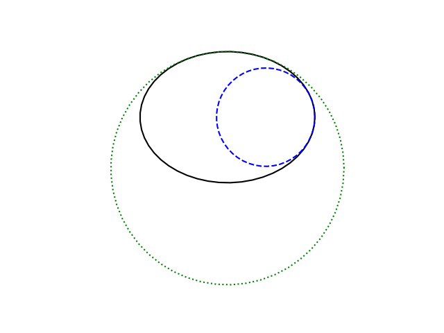
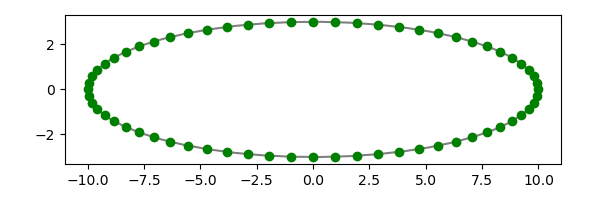
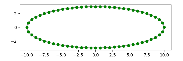
This equation is important because it essentially tells us how to locate an object in an elliptical orbit. M is mean anomaly, e is eccentricity, and E is eccentric anomaly. Mean anomaly is essentially time. Eccentric anomaly is not exactly the position of the orbiting object, but the position can be easily derived from E. See these notes on mean anomaly and eccentric anomaly. This is because we’re using our increased computing power to track more objects, such as debris in low earth orbit or things that might impact Earth some day.

Newton’s method

A fairly obvious approach to solving Kepler’s equation is to use Newton’s method. I think Newton himself applied his eponymous method to this equation.

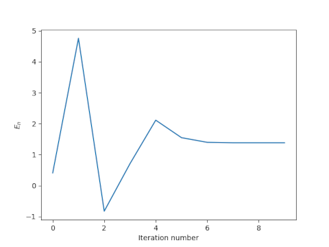
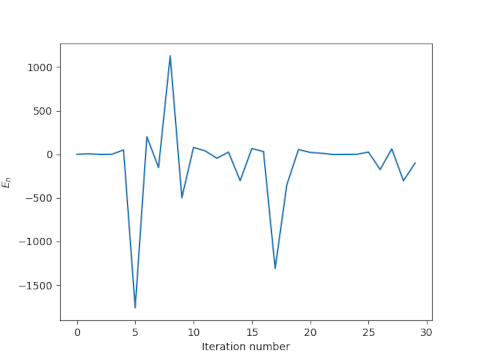
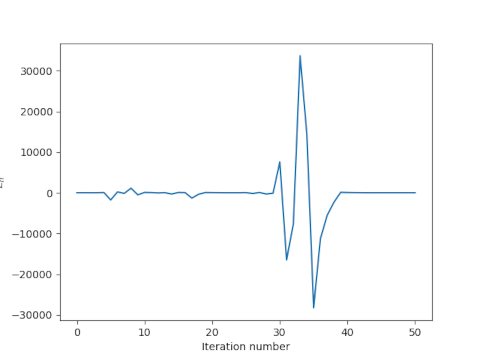
Newton’s method is very efficient when it works. As it starts converging, the number of correct decimal places doubles on each iteration. The problem is, however, that it may not converge. When I taught numerical analysis at Vanderbilt, I used a textbook that quoted this nursery rhyme at the beginning of the chapter on Newton’s method.

There was a little girl who had a little curl
Right in the middle of her forehead.
When she was good she was very, very good
But when she was bad she was horrid.

To this day I think of that rhyme every time I use Newton’s method. When Newton’s method is good, it is very, very good, converging quadratically. When it is bad, it can be horrid, pushing you far from the root, and pushing you further away with each iteration. Finding exactly where Newton’s method converges or diverges can be difficult, and the result can be quite complicated. Some fractals are made precisely by separating converging and diverging points.

Newton’s method solves f(x) = 0 by starting with an initial guess x₀ an iteratively applies

$x_{n+1} = x_n - \frac{f(x_n)}{f'(x_n)}$

Notice that

A sufficient condition for Newton’s method to converge is for x₀ to belong to a disk around the root where

$\left| \frac{f(x)f''(x)}{f'(x)^2}\right| < 1$

throughout the disk.

In our case f is the function

$f(x; e, M) = x - e \sin(x) - M$

where I’ve used x instead of E because Mathematica reserves E for the base of natural logarithms. To see whether the sufficient condition for convergence given above applies, let’s define

$g(x; e, M) = \left| \frac{e(x - e \sin x - M) \sin x}{(1 - e\cos x)^2} \right|$

Notice that the denominator goes to 0 as e approaches 1, so we should expect difficulty as e increases. That is, we expect Newton’s method might fail for objects in a highly elliptical orbit. However, we are looking at a sufficient condition, not a necessary condition. As I noted here, I used Newton’s method to solve Kepler’s equation for a highly eccentric orbit, hoping for the best, and it worked.

Starting guess

Newton’s method requires a starting guess. Suppose we start by setting E = M. How bad can that guess be? We can find out using Lagrange multipliers. We want to maximize

subject to the constraint that E and E satisfy Kepler’s equation. (We square the difference to get a differentiable objective function to maximize. Minimizing the squared difference minimizes the absolute difference.)

Lagrange’s theorem tells us

$\begin{pmatrix} 2x \\ -2M\end{pmatrix} = \lambda \begin{pmatrix} 1 - e \cos x \\ -1\end{pmatrix}$

and so λ = 2M and

$2x = 2M(1 - e\cos x)$

We can conclude that

$|x - M| \leq \frac{|e \cos x|}{2} \leq \frac{e}{2} \leq \frac{1}{2}$

This says that an initial guess of M is never further than a distance of 1/2 from the solution x, and its even closer when the eccentricity e is small.

If e is less than 0.55 then Newton’s method will converge. We can verify this in Mathematica with

    NMaximize[{g[x, e, M], 0 < e < 0.55, 0 <= M <= Pi, 
        Abs[M - x] < 0.5}, {x, e, M}]

which returns a maximum value of 0.93. The maximum value is an increasing function of the upper bound on e, so converting for e = 0.55 implies converging for e < 0.55. On the other hand, we get a maximum of 1.18 when we let e be as large as 0.60. This doesn’t mean Newton’s method won’t converge, but it means our sufficient condition cannot guarantee that it will converge.

A better starting point

John Machin (1686–1751) came up with a very clever, though mysterious, starting point for solving Kepler’s equation with Newton’s method. Machin didn’t publish his derivation, though later someone was able to reverse engineer how Machin must have been thinking. His starting point is as follows.

$\begin{align*} n &= \sqrt{5 + \sqrt{16 + \frac{9}{e}}} \\ M &= n \left((1-e)s + \frac{e(n^2 - 1) + 1}{6}s^3 \right) \\ x_0 &= n \arcsin s \end{align*}$

This produces an adequate starting point for Newton’s method even for values of e very close to 1.

Notice that you have to solve a cubic equation to find s. That’s messy in general, but it works out cleanly in our case. See the next post for a Python implementation of Newton’s method starting with Machin’s starting point.

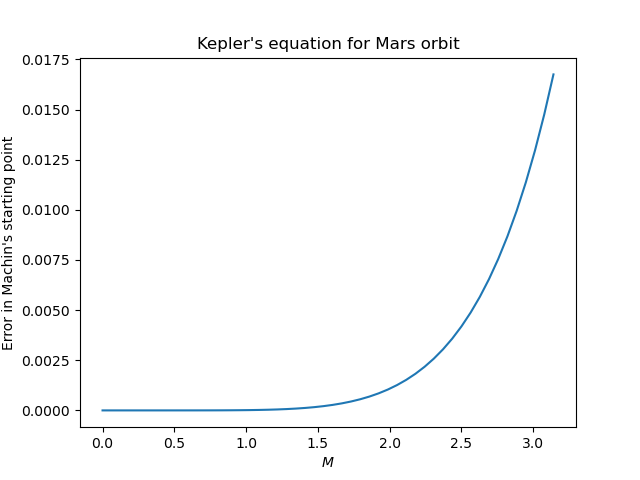
There are simpler starting points that are better than starting with M but not as good as Machin’s method. It may be more efficient to spend less time on the best starting point and more time iterating Newton’s method. On the other hand, if you don’t need much accuracy, and e is not too large, you could use Machin’s starting point as your final value and not use Newton’s method at all. If e < 0.3, as it is for every planet in our solar system, then Machin’s starting point is accurate to 4 decimal places (See Appendix C of Colwell’s book).

The fish curve

The electric motor curve

The ampersand curve

Related posts

GFSR

Pentanomial

Primitive polynomials

Practicalities

Related links

Related posts

Nephroid curve

Cayley’s sextit

Algebra

Nephroid evolute

Cayley’s sextit evolute

Kissing circles

Equation of evolute

Similar posts

The Good

The Bad

The Ugly

Commentary

Related posts

Special case: quarter of an ellipse

General case

Python code

Kepler’s equation

Newton’s method

Starting guess

A better starting point