ASCII armor: send encrypted data in plain text

GnuPG ASCII armor is a way to encode binary data as text and decode the text back into binary. It could be used with any binary data, but most often it is used with cryptographic data: public keys, encrypted messages, etc.

Secure communication over an insecure channel

When people ask whether some medium “supports encryption,” or more specifically whether the medium “supports end-to-end encryption,” they’re asking how convenient it is to use the medium with encrypted data. Any medium can convey encrypted text, but the process may be more or less manual.

You can use Gmail for end-to-end encryption, for example, though I’m sure Google would rather you not. Just encrypt the data on your computer, convert the output to ASCII, paste it into an email, and send. The receiver then copies the ASCII text, converts it to binary, and then decodes it.

ASCII armor is a way of handling the conversion to and from ASCII, with some niceties such as a checksum and human-friendly formatting, as friendly as formatting can be under the circumstances.

Aside: Coding versus Encryption

There are two kinds of encoding in this context: secret and non-secret. Coding theory is often misunderstood because it is primarily concerned with non-secret encoding, such as error-correcting codes and transmission protocols. ASCII armor belongs to coding theory, not encryption, though it is usually deployed in service of encryption.

ASCII armor is not providing protection from prying eyes. It is providing a relatively convenient way to convey naturally binary data, including a checksum to detect errors in transmission.

How ASCII armor works

At its heart, ASCII armor does base-64 encoding. But there’s more to it than that. There are optional fields, formatting rules, and a checksum.

For an example, we’ll take the first 120 binary digits of π after the “decimal” point.

Here’s some Python code to write the bits to a file. We start with the bits in hexadecimal since that’s more compact. In hex notation, π = 3.243f6a8885a3… For more details, see this post on hexadecimal floating point.

import binascii

data = '243F6A8885A308D313198A2E03707344A4093822299F31D0082EFA98EC4E6C89'
with open('pibits', 'wb') as f:
    f.write(binascii.unhexlify(data))

We can inspect pibits in a hex editor to verify that the bits are correct, say by running xxd.

Enarmor

We can convert our binary file to ASCII using gpg, which stands for GNU Privacy Guard (GnuPG), the GNU implementation of Pretty Good Privacy. Running

gpg --enarmor pibits

produces a file pibits.ascii with the following contents.

-----BEGIN PGP ARMORED FILE-----
Comment: Use "gpg --dearmor" for unpacking

JD9qiIWjCNMTGYouA3BzRKQJOCIpnzHQCC76mOxO
=0G7A
-----END PGP ARMORED FILE-----

Dearmor

If we run

gpg --dearmor pibits.asc

we get a file pibits.asc.gpg identical to the original file pibits, which we could verify using diff.

Base 64 encoding

How does the string JD9… above correspond to bits?

A hexadecimal character represents 4 bits, and a base 64 character represents 6 bits. So every 3 hexadecimal character corresponds to 12 bits or 2 base 64 characters.

The first three hexadecimal characters in our data, 243, corresponds to the first two characters in our ASCII armor data, JD, as follows. First of all,

243hex = 001001000011two

and if we split the bits into groups of six we have 001001two = 9ten and 000011two = 3ten. ASCII armor represents base-64 numbers the same way MIME encoding does: the numbers 0 through 63 are represented by

A, B, C, … Z, a, b, c, …, z, 0, 1, 2, …, 9, +, /

So 9 is encoded as J, and 3 is encoded as D.

The 120 bits of π represented by the 30 hexadecimal characters 243…C89 or by the 20 base 64 characters JD…xO in base 64. Note that the last character is the letter O, not the decimal 0. (Base 58 avoids this problem by not using typographically similar symbols.)

In this example we had 120 bits, which is a multiple of 6. What if the number of bits is not a multiple of 6? See this post for an answer.

Checksum

After the 20 characters encoding our data follows five more characters, =0G7A. The equal sign is a separator, and 0G7A is a base 64 encoding of a 24-bit CRC checksum. The details of the checksum, and C code for implementing it, are given in RFC 4880 Section 6.1.

Related posts

Why not reuse passwords?

Perhaps you’ve heard that you should not reuse passwords but don’t understand why. After all, you have a really good password, one that nobody would ever guess, so why not use it everywhere?

Your password is not as good as you think

First of all, people who think they have a really good password are usually wrong. They implicitly assume that an attacker would have to recreate the devious process they went through to create the password. This is not the case. A password needs to be hard for an attacker to crack, not hard for the owner to create, and these are not the same thing. The former requires passwords that are long and randomly generated.

Credential stuffing

Suppose you use the same password on sites X and Y. Then site X gets hacked, revealing your password. Now your user name (most likely your email address) and password is part of a list posted online somewhere. Hackers then use scripts to see whether the same credentials will work somewhere else, and they often do. If they try site Y, then your account on Y has been compromised as well.

Now suppose you use a different username at the two sites. This is better, but the hack on X still means that your password has been added to a list of known passwords.

The worst case scenario is a site that stores passwords in the clear. This practice has long been discouraged, but the more times you reuse a password, the higher the chance that you’ll use your password at a site that does not hash passwords.

Hashing

Most sites these days don’t store your password per se but a cryptographic hash of your password. When you enter your password, the site hashes it and compares the result to the hashed value it has on file. If they match, you’re in.

If your hashed password for X is part of a breach, and the hashing algorithms for X and Y known, an attacker can try hashing a list of known passwords and maybe one of them will match the hash of your password on Y.

If sites X and Y use different hashing algorithms, then a hash of your password for X is not directly useful to hacking your account on site Y. But it is possible to “unhash” passwords, especially if a site uses a hashing algorithm that has been broken. This takes a lot of computation, but people do it.

Example

This is not hypothetical. It has happened many times. For example, it was part of what lead to the recent 23andMe breach. And when a hacker obtains one person’s family tree data, they obtain data on many other people at the same time. If you used a unique, long, randomly generated password on 23andMe but your cousin used password123, then your data may have been stolen.

What to do?

What can you do? You almost have to use a password manager. A strong password is necessarily hard to remember, and memorizing hundreds of strong passwords would be quite a chore. Still, you might want to memorize one or two strong passwords if they protect something really valuable.

Related posts

The world’s sneakiest substitution

Something that seems like an isolated trick may turn out to be much more important. This is the case with a change of variables discovered by Karl Weierstrass.

Every calculus student learns a handful of standard techniques: u-substitutions, partial fractions, integration by parts, and trig substitutions. Then there is one more technique that is like something off a secret menu, something know only to the cognoscenti: Weierstrass’ t = tan(x/2) trick [1]. Michael Spivak called this “the world’s sneakiest substitution.”

The world's sneakiest substitution is undoubtedly t = tan(x/2), x = 2 arctan t, dx = 2 dt / (1 + t^2)

This was on page 325 of the first edition of Spivak’s Calculus, page 360 of the second edition.

This innocent but apparently unmotivated change of variables has the following magical consequences:

  • sin(x) = 2t/(1 + t2)
  • cos(x) = (1 – t2) / (1 + t2)
  • dx = 2 dt/(1 + t2).

This means that the trick can convert an integral containing any rational combination of trig functions into one involving only rational functions, which then can (in principle) be integrated in closed form using partial fractions. It’s the key that unlocks all trig integrals.

However, this is not as practical as it sounds. You may get a high-degree rational function, and while in theory the rational function can be integrated using partial fractions, the decomposition may be tedious if not impossible. Still, it’s interesting that a single trick reduces one large class of integration problems to another.

Now let’s leave integration behind. The equations above say that as t varies, the functions 2t/(1 + t2) and (1 – t2) / (1 + t2) take on all the values that sin(x) and cos(x) do. This means, for example, that you can draw a circle using graphics hardware that does not support sines and cosines. In theory the range of t would have to be infinite, but in practice the range would only have to be large enough to fill in the right pixels.

If we can parameterize a circle with rational functions, what else can we parameterize this way? It turns out, for example, that elliptic curves do not have rational parameterizations. This question is its own niche of algebraic geometry. I don’t know the history here, but it’s plausible some of this math was motivated by wondering what else could be done along the lines of Weierstrass’ trick.

[1] When I’ve mentioned this trick before, some have told me this was a routine part of their course. That was not my experience, either as a student or as an instructor. As a freshman I learned the trick from a friend who was the best of our cohort at integration, someone who would have done well at an integration bee if we’d had one. I felt I’d been let in on a secret.

f(g(x)) versus g(f(x))

I stumbled upon a theorem today that I feel like I’ve needed in the past, though I can’t remember any particular applications. I’m writing it up here as a note to my future self should the need reappear.

The theorem gives sufficient conditions to conclude

f(g(x)) ≤ g(f(x))

and uses this to prove, for example, that

arcsin( sinh(x/2) ) ≤ sinh( arcsin(x)/2 )

on the interval [0, 1].

If you think of any applications, please leave a comment.

Here’s the theorem, found in [1].

Let f be continuous with domain 0 ≤ x < 1 or 0 ≤ x ≤ 1, f(0) = 0, f(1) > 1 (including the possibility that f(1) = +∞); let g be continuous with domain the range of f, and g(1) ≤ 1. Let f(x)/x and g(x)/x be strictly increasing on their domains. Finally let f(x) ≠ x for 0 < x < 1. Then f(g(x)) ≤ g(f(x)) for 0 < x < 1.

[1] Ralph P. Boas. Inequalities for a Collection. Mathematics Magazine, January 1979, Vol. 52, No. 1, pp. 28–31

Constellations in Mathematica

Mathematica has data on stars and constellations. Here is Mathematica code to create a list of constellations, sorted by the declination (essentially latitude on the celestial sphere) of the brightest star in the constellation.

constellations = EntityList["Constellation"]
sorted = SortBy[constellations, -#["BrightStars"][[1]]["Declination"] &]

We can print the name of each constellation with

Map[#["Name"] &, sorted]

This yields

{"Ursa Minor", "Cepheus", "Cassiopeia", "Camelopardalis", 
…, "Hydrus", "Octans", "Apus"}

We can print the name of the constellation along with its brightest star as follows.

Scan[Print[#["Name"], ", " #["BrightStars"][[1]]["Name"]] &, sorted]

This prints

Ursa Minor, Polaris
Cepheus, Alderamin
Cassiopeia, Tsih
Camelopardalis, β Camelopardalis
…
Hydrus, β Hydri
Octans, ν Octantis
Apus, α Apodis

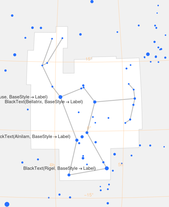
Mathematica can draw star charts for constellations, but when I tried

Entity["Constellation", "Orion"]["ConstellationGraphic"]

it produced extraneous text on top of the graphic.

Related posts

222nd Carnival of Mathematics

A blog carnival is a round up of recent blog posts. The Carnival of Mathematics is a long-running carnival of blog posts on mathematical topics. This is the 222nd edition of the carnival.

Facts about 222

By longstanding tradition, the nth Carnival of Mathematics must begin with trivia about the number n, and so here are five facts about the number 222.

  • There are six groups of order 222, and 222 groups of order 912.
  • 222=9+87+6×5×4+3+2+1.
  • You can encode the number 222 in the Major mnemonic system as “unknown” or “one-on-one.”

The posts

Gil Kalai looks at what happens when you ask ChatGPT to solve Elchanan Mossel’s dice problem.

Γιώργος Πλούσος (@plousos2505 on the social media platform formerly know as Twitter) posted an image showing how to compute π via a sequence of approximations requiring only basic geometry.

David Eppstein’s blog 11011110 has a post on Pyramidology. It’s particularly fitting to have a post from 1101110 in this carnival. As the author explains in his About page,

This journal’s name comes from interpreting my initials as the hexadecimal number 0xDE (decimal 222) and then converting the result to binary.

The blog ThatsMaths has a post on Sharkovsky numbering, Oleksandr Sharkovsky (1936–2022), and Sharkovsky’s Theorem. This post includes the beautiful image from Wikimedia.

The post Patterns of reality by Timothy Williamson gives an overview of logic from basics to the work of Gödel and Turing.

Larissa Fedunik-Hofman posts an interview with Andrew Krause discussing dynamical system.

Finally, we have Matthew Scroggs’ Advent calendar of math puzzles.

To see previous editions of the carnival, or to submit a post to the next edition, see the Carnival of Mathematics page on Aperiodical.

Bounding complex roots by a positive root

Suppose you have an nth degree polynomial with complex coefficients

p(z) = anzn + an-1zn-1 + … + a0

and you want to find some circle that is guaranteed to contain all the zeros of p.

Cauchy found such a circle in 1829. The zeros of p lie inside the circle |z| ≤ r where r is the unique positive root of

f(z) = |an|zn − |an-1|zn-1 − … − |a0|

This value of r is known as the Cauchy radius of the polynomial p.

This may not seem like much of an improvement: you started with wanting to find the roots of an nth degree polynomial and you end with finding the roots of an nth degree polynomial. But Cauchy’s theorem reduces the problem of finding all roots of a complex polynomial to finding one root of a real polynomial. Furthermore, the positive root we’re after is guaranteed to be unique.

If a0 = 0 then p(z) has a factor of z and so we can reduce the problem to bounding the zeros of p(z)/z. Otherwise, f(0) < 0. Eventually f(z) must be positive because the zn term will overtake the rest of the terms for large enough z. So we only need to find some value of z where f(z) > 0 and then we could use the bisection method to find r.

Since our goal is to bound the zeros of p, we don’t need to find r exactly: an upper bound on r will do, though the smaller the upper bound the better. The bisection method gives us a sequence of upper bounds, so we could work in rational arithmetic and have rigorously provable upper bounds.

As for how to find a real value of z where f is positive, we could try z = 2k for successive value of k until we find one that works.

For example, let’s bound the roots of

p(z) = 12z5 + 2z2 + 23i = 0.

Cauchy’s theorem says we need to find the unique positive root of

f(z) = 12z5 − 2z2 − 23.

Now f(0) = −23 and f(2) = 353. So we know right away that the roots of p have absolute value less than 2.

Next we evaluate f(1), which turns out to be −13, and so the Cauchy radius is larger than 1. This doesn’t necessarily mean that p has a root with absolute value greater than 1, only that the Cauchy radius is greater than 1. An upper bound on the Cauchy radius is an upper bound on the absolute values of the roots of p; a lower bound on the Cauchy radius is not necessarily a lower bound on the largest root.

Carrying out two steps of the bisection method by hand was easy, but let’s automate the process of carrying it out further.

>>> from scipy.optimize import bisect
>>> bisect(lambda x: 12*x**5 - 2*x*x - 23, 1, 2)
1.1646451258329762

So Python tells us r = 1.1646451258329762.

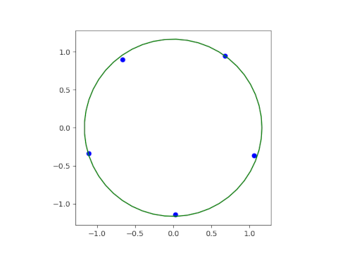
Here’s a plot of the roots and the Cauchy radius.

In this example the roots of p are located very near a circle with the Cauchy radius. The roots range in absolute value between 1.1145600699993699 and 1.1634197192917954. The roots nearly lie in a circle because the quadratic term in our polynomial is small and so we are approximately finding the fifth roots of −23i.

Let’s do another example with randomly generated coefficients to get a better idea of how Cauchy’s theorem works in general. The coefficients of our polynomial, from 0th to 5th, are

0.126892 + 0.689356i,  -0.142366 + 0.260969, – 0.918873 + 0.489906i,  0.0599824 – 0.679312i,  – 0.222055 + 0.273651, + 0.154408 + 0.733325i

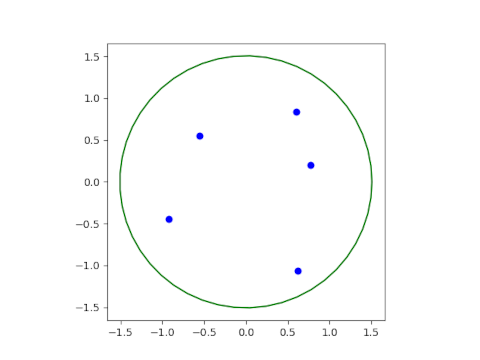
The roots have absolute value between 0.7844606228243709 and 1.2336256274024142, and the Cauchy radius is 1.5088421845957782. Here’s a plot.

Related posts

Convergent subsequence

I was reading a theorem giving conditions for a divergent series to have a convergent subseries and had a sort of flashback.

I studied nonlinear PDEs in grad school, which amounted to applied functional analysis. We were constantly proving or using theorems about sequences having convergent subsequences, often subsequences that converged in a very weak sense.

This seemed strange to me at first. If a sequence diverges, why is it of any interest that a subsequence converges? This seemed like blackout poetry, completely changing the meaning of a text by selecting various words. For example, here is the opening paragraph of Pride and Prejudice, blacked out to appear to be a real estate ad.

good neighborhood, surrounding park

Here’s the big picture I was missing. We’re trying to show that a differential equation has a solution, and we’re doing that by some kind of successive approximation. Maybe our series of approximations doesn’t work in general, but that doesn’t matter. We’re just trying to find something that is a solution. Once you come up with a candidate solution, by whatever means, grasping at whatever straws you can grasp, you then prove that the candidate really is a solution, perhaps a solution in a weak sense. Then you show that this solution, potentially one of many, is unique. Then you show that your weak solution is a in fact a solution in a stronger sense.

Related posts

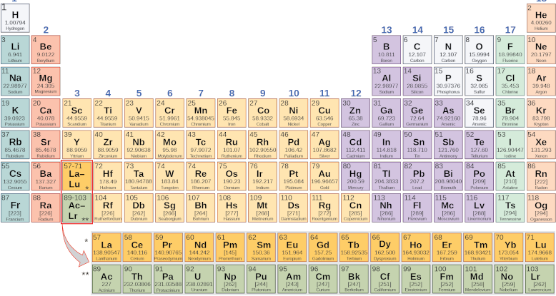
How to memorize the periodic table

Periodic table image

Motivation

Memorizing the periodic table has some practical value, especially if you’re a chemist, but in any case it’s an interesting exercise, easier to do than it may sound. And it’s a case study for how you might memorize other things of more practical value to you personally.

Major system pegs

The Major system is a way to associate consonant sounds to numbers. You can fill in vowels and semivowels as you please to turn the sequence of consonant sounds into words, preferably words that create a vivid image in your mind.

You can pick a canonical encoding of each number to create a set of pegs and use these to memorize numbered lists. Although numbers can be encoded many ways, a set of pegs is a one-to-one mapping to numbers. To pull up the nth item in the list, recall what image you’ve associated with the peg image for n.

For example, you could encode 16 as dish, tissue, touché, Hitachi, etc. If you want to remember that sulfur has atomic number 16 you could use any of those images. But if you wanted to remember that the 16th element is sulfur, you need to have a unique peg associated with 16.

Learning pegs is more work than hanging things on pegs. But once you have a set of pegs, you can reuse them for memorizing multiple lists. For example, you could use the same pegs to memorize the periodic table and the ASCII table.

Atomic numbers

Allan Krill has written up a way to associate each element with a peg. You could use his suggestions, but you’ll almost certainly need to customize some of them. It’s generally hard to use anyone else’s mnemonics. What works for one person may not for another.

To memorize the periodic table, you first come up with pegs for the numbers 1 through 118. Practice those and get comfortable with them. This could take a while, but it’s reusable effort. Then associate an image of each element with its corresponding peg. For example, polonium is element 84. If your peg for 84 is fire, you might imagine someone playing polo on a field that’s on fire.

Element symbols

Every element has a one- or two-letter symbol, and most of these are easy: Ti for titanium, U for uranium, etc. Some seem completely arbitrary, such as Hg for mercury, but these you may already know. These names seem strange because they are mnemonic in Latin. But the elements with Latin names are also the ones that were discovered first and are the most common. You probably know by osmosis, for example, that the symbol for iron is Fe.

The hard part is the second letter, if there is a second letter. For example, is does Ar stand for argon or arsenic? Is the symbol for thulium Th or Tl or Tm?

When you associate an element image with a peg image, you could add a third image for the second letter of the element symbol, using the NATO phonetic alphabet if you know that. For example, the NATO word for S is Sierra. If your peg for 33 is mummy, you might imagine a mummy drinking a bottle of Sierra Springs® water laced with arsenic.

Related posts

Image from OpenStax Biology 2e. CC BY Attribution license.

Solving a triangle the size of Argentina

The numbers in today’s date—11, 28, and 23—make up the sides of a triangle. This doesn’t always happen; the two smaller numbers have to add up to more than the larger number.

We’ll look at triangles with sides 11, 23, and 28 in the plane, on a sphere, and on a hypersphere. Most of the post will be devoted to the middle case, a large triangle on the surface of the earth.

Solving a triangle in the plane

If we draw a triangle with sides 11, 23, and 28, we can find out the angles of the triangle using the law of cosines:

c² = a² + b² – 2ab cos C

where C is the angle opposite the side c. We can find each of the angles of the triangle by rotating which side we call c.

If we let c = 11, then C = arccos((23² + 28² − 11²)/(2 × 23 × 28)) = 22.26°.

If we let c = 23, then C = arccos((11² + 28² − 23²)/(2 × 11 × 28)) = 52.38°.

If we let c = 28, then C = arccos((11² + 23² − 28²)/(2 × 11 × 23)) = 105.36°.

Solving a triangle on a sphere

Now suppose we make our 11-23-28 triangle very large, drawing our triangle on the face of the earth. We pick our unit of measurement to be 100 miles, and we get a triangle very roughly the size and shape of Argentina.

We can still use the law of cosines, but it takes a different form, and the meaning of the terms changes. The law of cosines on a sphere is

cos(c) = cos(a) cos(b) + sin(a) sin(b) cos(C).

As before, a, b, and c are sides of the triangle, and the sides b and c intersect at an angle C. However, now the sides themselves are angles because they are arcs on a sphere. Now a, b, and c are measured in degrees or radians, not in miles.

If the length of an arc is x, the angular measure of the arc is 2πx/R where R is the radius of the sphere. The mean radius of the earth is 3959 miles, and we’ll assume the earth is a sphere with that radius.

We can solve for the angle opposite the longest side by using

C = arccos( (cos(c) – cos(a) cos(b)) / sin(a) sin(b) )

where

a = 2π × 1100 / 3959
b = 2π × 2300 / 3959
c = 2π × 2800 / 3959

It turns out that C = 149.8160°, and the other angles are 14.3977° and 29.4896°.

Importantly, the sum of these three angles is more than 180°. In fact it’s 193.7033°.

The sum of the vertex angles in a spherical triangle is always more than 180°, and the bigger the triangle, the more the sum exceeds 180°. The amount by which the sum exceeds 180° is called the spherical excess E and it is proportional to the area. In radians,

E = area / R².

In our example the excess is 13.7033° and so the area of our triangle is

13.7033° × (π radians / 180°) × 3959² miles² = 3,749,000 miles².

Now Argentina has an area of about a million square miles, so our triangle is bigger than Argentina, but smaller than South America (6.8 million square miles). Argentina is about 2300 miles from north to south, so one of the sides of our triangle matches Argentina well.

Note that there are no similar triangles on a sphere: if you change the lengths of the sides proportionately, you change the vertex angles.

Solving a triangle on a pseudosphere

In a hyperbolic space, such as the surface of a pseudosphere, a surface that looks sorta like the bell of a trombone, the law of cosines becomes

cosh(c) = cosh(a) cosh(b) + κ sinh(a) sinh(b) cos(C)

where κ < 0 is the curvature of the space. Note that if we set κ = 1 and delete all the hs this would become the law of cosines on a sphere.

Just as the sum of the angles in a triangle add up to more than 180° on a sphere, and exactly 180° in a plane, they add up to less than 180° on a pseudosphere. I suppose you could call the difference between 180° and the sum of the vertex angles the spherical deficiency by analogy with spherical excess, but I don’t recall hearing that term used.

Related posts