Hallucinations of AI Science Models

AlphaFold 2, FourCastNet and CorrDiff are exciting. AI-driven autonomous labs are going to be a big deal [1]. Science codes now use AI and machine learning to make scientific discoveries on the world’s most powerful computers [2].

It’s common practice for scientists to ask questions about the validity, reliability and accuracy of the mathematical and computational methods they use. And many have voiced concerns about the lack of explainability and potential pitfalls of AI models, in particular deep neural networks (DNNs) [3].

The impact of this uncertainty varies highly according to project. Science projects that are able to easily check AI-generated results against ground truth may not be that concerned. High-stakes projects like design of a multimillion dollar spacecraft with high project risks may ask about AI model accuracy with more urgency.

Neural network accuracy

Understanding of the properties of DNNs is still in its infancy, with many as-yet unanswered questions. However, in the last few years some significant results have started to come forth.

A fruitful approach to analyzing DNNs is to see them as function approximators (which, of course, they are). One can study how accurately DNNs approximate a function representing some physical phenomenon in a domain (for example, fluid density or temperature).

The approximation error can be measured in various ways. A particularly strong measure is “sup-norm” or “max-norm” error, which requires that the DNN approximation be accurate at every point of the target function’s domain (“uniform approximation”). Some science problems may have a weaker requirement than this, such as low RMS or 2-norm error. However, it’s not unreasonable to ask about max-norm approximation behaviors of numerical methods [4,5].

An illuminating paper by Ben Adcock and Nick Dexter looks at this problem [6]. They show that standard DNN methods applied even to a simple 1-dimensional problem can result in “glitches”: the DNN as a whole matches the function well but at some points totally misapproximates the target function. For a picture that shows this, see [7].

Other mathematical papers have subsequently shed light on these behaviors. I’ll try to summarize the findings below, though the actual findings are very nuanced, and many details are left out here. The reader is advised to refer to the respective papers for exact details.

The findings address three questions: 1) how many DNN parameters are required to approximate a function well? 2) how much data is required to train to a desired accuracy? and 3) what algorithms are capable of training to the desired accuracy?

How many neural network weights are needed?

How large does the neural network need to be for accurate uniform approximation of functions? If tight max-norm approximation requires an excessively large number of weights, then use of DNNs is not computationally practical.

Some answers to this question have been found—in particular, a result 1 is given in [8, Theorem 4.3; cf. 9, 10]. This result shows that the number of neural network weights required to approximate an arbitrary function to high max-norm accuracy grows exponentially in the dimension of the input to the function.

This dependency on dimension is no small limitation, insofar as this is not the dimension of physical space (e.g., 3-D) but the dimension of the input vector (such as the number of grid cells), which for practical problems can be in the tens [11] or even millions or more.

Sadly, this rules out the practical use of DNN for some purposes. Nonetheless, for many practical applications of deep learning, the approximation behaviors are not nearly so pessimistic as this would indicate (cp. [12]). For example, results are more optimistic:

  • if the target function has a strong smoothness property;
  • if the function is not arbitrary but is a composition of simpler functions;
  • if the training and test data are restricted to a (possibly unknown) lower dimensional manifold in the high dimensional space (this is certainly the case for common image and language modeling tasks);
  • if the average case behavior for the desired problem domain is much better than the worst case behavior addressed in the theorem;
  • The theorem assumes multilayer perceptron and ReLU activation; other DNN architectures may perform better (though the analysis is based on multidimensional Taylor’s theorem, which one might conjecture applies also to other architectures).
  • For many practical applications, very high accuracy is not a requirement.
  • For some applications, only low 2-norm error is sufficient, (not low max-norm).
  • For the special case of physics informed neural networks (PINNs), stronger results hold.

Thus, not all hope is lost from the standpoint of theory. However, certain problems for which high accuracy is required may not be suitable for DNN approximation.

How much training data is needed?

Assuming your space of neural network candidates is expressive enough to closely represent the target function—how much training data is required to actually find a good approximation?

A result 2 is given in [13, Theorem 2.2] showing that the number of training samples required to train to high max-norm accuracy grows, again, exponentially in the dimension of the input to the function.

The authors concede however that “if additional problem information about [the target functions] can be incorporated into the learning problem it may be possible to overcome the barriers shown in this work.” One suspects that some of the caveats given above might also be relevant here. Additionally, if one considers 2-norm error instead of max-norm error, the data requirement grows polynomially rather than exponentially, making the training data requirement much more tractable. Nonetheless, for some problems the amount of data required is so large that attempts to “pin down” the DNN to sufficient accuracy become intractable.

What methods can train to high accuracy?

The amount of training data may be sufficient to specify a suitable neural network. But, will standard methods for finding the weights of such a DNN be effective for solving this difficult nonconvex optimization problem?

A recent paper [14] from Max Tegmark’s group empirically studies DNN training to high accuracy. They find that as the input dimension grows, training to very high accuracy with standard stochastic gradient descent methods becomes difficult or impossible.

They also find second order methods perform much better, though these are more computationally expensive and have some difficulty also when the dimension is higher. Notably, second order methods have been used effectively for DNN training for some science applications [15]. Also, various alternative training approaches have been tried to attempt to stabilize training; see, e.g., [16].

Prospects and conclusions

Application of AI methods to scientific discovery continues to deliver amazing results, in spite of lagging theory. Ilya Sutskever has commented, “Progress in AI is a game of faith. The more faith you have, the more progress you can make” [17].

Theory of deep learning methods is in its infancy. The current findings show some cases for which use of DNN methods may not be fruitful, Continued discoveries in deep learning theory can help better guide how to use the methods effectively and inform where new algorithmic advances are needed.

Footnotes

1 Suppose the function to be approximated takes d inputs and has the smoothness property that all nth partial derivatives are continuous (i.e., is in Cn(Ω) for compact Ω). Also suppose a multilayer perceptron with ReLU activation functions must be able to approximate any such function to max-norm no worse than ε. Then the number of weights required is at least a fixed constant times (1/ε)d/(2n).

2 Let F be the space of all functions that can be approximated exactly by a broad class of ReLU neural networks. Suppose there is a training method that can recover all these functions up to max-norm accuracy bounded by ε. Then the number of training samples required is at least a fixed constant times (1/ε)d.

References

[1] “Integrated Research Infrastructure Architecture Blueprint Activity (Final Report 2023),” https://www.osti.gov/biblio/1984466.

[2] Joubert, Wayne, Bronson Messer, Philip C. Roth, Antigoni Georgiadou, Justin Lietz, Markus Eisenbach, and Junqi Yin. “Learning to Scale the Summit: AI for Science on a Leadership Supercomputer.” In 2022 IEEE International Parallel and Distributed Processing Symposium Workshops (IPDPSW), pp. 1246-1255. IEEE, 2022, https://www.osti.gov/biblio/2076211.

[3] “Reproducibility Workshop: The Reproducibility Crisis in ML‑based Science,” Princeton University, July 28, 2022, https://sites.google.com/princeton.edu/rep-workshop.

[4] Wahlbin, L. B. (1978). Maximum norm error estimates in the finite element method with isoparametric quadratic elements and numerical integration. RAIRO. Analyse numérique, 12(2), 173-202, https://www.esaim-m2an.org/articles/m2an/pdf/1978/02/m2an1978120201731.pdf

[5] Kashiwabara, T., & Kemmochi, T. (2018). Maximum norm error estimates for the finite element approximation of parabolic problems on smooth domains. https://arxiv.org/abs/1805.01336.

[6] Adcock, Ben, and Nick Dexter. “The gap between theory and practice in function approximation with deep neural networks.” SIAM Journal on Mathematics of Data Science 3, no. 2 (2021): 624-655, https://epubs.siam.org/doi/10.1137/20M131309X.

[7] “Figure 5 from The gap between theory and practice in function approximation with deep neural networks | Semantic Scholar,” https://www.semanticscholar.org/paper/The-gap-between-theory-and-practice-in-function-Adcock-Dexter/156bbfc996985f6c65a51bc2f9522da2a1de1f5f/figure/4

[8] Gühring, I., Raslan, M., & Kutyniok, G. (2022). Expressivity of Deep Neural Networks. In P. Grohs & G. Kutyniok (Eds.), Mathematical Aspects of Deep Learning (pp. 149-199). Cambridge: Cambridge University Press. doi:10.1017/9781009025096.004, https://arxiv.org/abs/2007.04759.

[9] D. Yarotsky. Error bounds for approximations with deep ReLU networks. Neural Netw., 94:103–114, 2017, https://arxiv.org/abs/1610.01145

[10] I. Gühring, G. Kutyniok, and P. Petersen. Error bounds for approximations with deep relu neural networks in Ws,p norms. Anal. Appl. (Singap.), pages 1–57, 2019, https://arxiv.org/abs/1902.07896

[11] Matt R. Norman, “The MiniWeather Mini App,” https://github.com/mrnorman/miniWeather

[12] Lin, H.W., Tegmark, M. & Rolnick, D. Why Does Deep and Cheap Learning Work So Well?. J Stat Phys 168, 1223–1247 (2017). https://doi.org/10.1007/s10955-017-1836-5

[13] Berner, J., Grohs, P., & Voigtlaender, F. (2022). Training ReLU networks to high uniform accuracy is intractable. ICLR 2023, https://openreview.net/forum?id=nchvKfvNeX0.

[14] Michaud, E. J., Liu, Z., & Tegmark, M. (2023). Precision machine learning. Entropy, 25(1), 175, https://www.mdpi.com/1099-4300/25/1/175.

[15] Markidis, S. (2021). The old and the new: Can physics-informed deep-learning replace traditional linear solvers?. Frontiers in big Data, 4, 669097, https://www.frontiersin.org/articles/10.3389/fdata.2021.669097/full

[16] Bengio, Y., Lamblin, P., Popovici, D., & Larochelle, H. (2006). Greedy layer-wise training of deep networks. Advances in neural information processing systems, 19,  https://papers.nips.cc/paper_files/paper/2006/hash/5da713a690c067105aeb2fae32403405-Abstract.html

[17] “Chat with OpenAI CEO and Co-founder Sam Altman, and Chief Scientist Ilya Sutskever,” https://www.youtube.com/watch?v=mC-0XqTAeMQ&t=250s


The IQ Test That AI Can’t Pass

Large language models have recently achieved remarkable test scores on well-known academic and professional exams (see, e.g., [1], p. 6). On such tests, these models are at times said to reach human-level performance. However, there is one test that humans can pass but every AI method known to have been tried has abysmally failed.

The Abstraction and Reasoning Corpus (ARC) benchmark [2] was developed by François Chollet to measure intelligence in performing tasks never or rarely seen before. We all do tasks something like this every day, like making a complicated phone call to correct a mailing address. The test is composed of image completion problems similar to Raven’s Progressive Matrices but more complex. Given images A, B and C, one must identify the image D such that the relationship “A is to B as C is to D” holds. Sometimes several examples of the A:B relationship are given.

The problem is hard because the relationship patterns between A and B that humans could easily identify (for example, image shrinking, rotating, folding, recoloring, etc.) might be many, many different things—more than can easily be trained for. By construction, every problem is qualitatively, unpredictably different, so the common approach of training on the training set doesn’t work. Instead, bonafide reasoning on a new kind of problem for each case is required.

Several competitions with prize money have encouraged progress on the ARC benchmark [3]. In these, each entrant’s algorithm must be tested against an unseen ARC holdout set. The leaderboard for the ARCathon 2023 challenge completed last month shows top score of 30 percent [4]; this is excellent progress on a very hard problem, but far from a perfect score or anything else resembling passing.

Ilya Sutskever has famously warned we shouldn’t bet against deep learning, and perhaps a future LLM will do much better on this benchmark. Others feel a new approach is needed, for example, from the burgeoning field of neurosymbolic methods. In any case, these results show at the present moment in this rapidly progressing field, we don’t seem to be anywhere close to strong forms of AGI, artificial general intelligence.

[1] OpenAI, “GPT-4 Technical Report,” https://cdn.openai.com/papers/gpt-4.pdf

[2] François Chollet, “On the Measure of Intelligence,” https://arxiv.org/abs/1911.01547

[3] “Abstraction and Reasoning Challenge,” https://www.kaggle.com/c/abstraction-and-reasoning-challenge

[4] “Winners – Lab42, “https://lab42.global/winners/

The Million Dollar Matrix Multiply

The following post is by Wayne Joubert, the newest member of our consulting team. Wayne recently retired from his position as a Senior Computational Scientist at Oak Ridge National Laboratory. — John

Training large language models like GPT-4 costs many millions of dollars in server expenses. These costs are expected to trend to billions of dollars over the next few years [1]. One of the biggest computational expenses of LLM training is multiplying matrices. These are simple operations of the form C = AB. Matrix multiplies are common not only in AI model training but also many high performance computing applications from diverse science domains.

Eking out more speed from matrix multiplies could reduce AI model training costs by millions of dollars. More routinely, such improvements could reduce training runtime by hours on a single GPU-powered workstation or cut down cloud service provider expenses significantly.

What is less well-known is that matrix multiples run on graphics processing units (GPUs) that are typically used for model training have many exotic performance behaviors that can drastically reduce matrix multiply efficiency by a wide margin.

Two recent works [2], [3] examine these phenomena in considerable depth. Factors such as matrix size, alignment of data in memory, power throttling, math library versions, chip-level manufacturing variability, and even the values of the matrix entries can significantly affect performance. At the same time, much of this variability can be modeled by machine learning methods such as decision trees and random forests [2].

Use of these methods can be the first step toward implementing autotuning techniques to minimize costs. Using such methods or carefully applying rules of thumb for performance optimization can make a huge performance difference for matrix multiply-heavy GPU software.

Related posts

[1] What large models cost you—there is no free AI lunch

[2] Wayne Joubert, Eric Palmer and Verónica G. Melesse Vergara, “Matrix Multiply Performance of GPUs on Exascale-class HPE/Cray Systems,” Proceedings of the Cray User Group Meeting (CUG) 2022, https://www.osti.gov/biblio/2224210.

[3] P. Sinha, A. Guliani, R. Jain, B. Tran, M. D. Sinclair and S. Venkataraman, “Not All GPUs Are Created Equal: Characterizing Variability in Large-Scale, Accelerator-Rich Systems,” SC22: International Conference for High Performance Computing, Networking, Storage and Analysis, Dallas, TX, USA, 2022, pp. 01-15, doi: 10.1109/SC41404.2022.00070.

Differentially private stochastic gradient descent

Let’s work our way up to differentially private stochastic gradient descent (DP-SGD) a little at a time. We’ll first look at gradient descent, then stochastic gradient descent, then finally differentially private stochastic gradient descent.

Gradient descent

We’ll start with gradient descent. Suppose you have a function of several variables f(x) where x is a vector. Then the gradient ∇f(x) points in the direction of greatest increase in f, and its negative −∇f(x) points in the direction of greatest decrease. So you can decrease the function f by moving in the direction −∇f(x). You can turn this observation into an algorithm for minimizing f. Find the gradient, take a step in the opposite direction. Rinse, lather, and repeat. The gradient descent method is also called steepest descent because locally you’re always moving in the direction of steepest descent.

Locally is the key word here. In some finite neighborhood of x, −∇f(x) points in a direction that will decrease the value of f. How large is this neighborhood? Hard to say. How long a step should you take? Also hard to say.

If your function f is strictly convex, then there is a global minimum, and the gradient descent algorithm will converge to it.

Stochastic gradient descent

What could go wrong? If your objective function f is strictly convex, convergence is guaranteed, but convergence may be slow. The method is always locally optimal, but optimal may mean inside a tiny little neighborhood of where you start each iteration.

Gradient descent can meander through a valley, a nearly flat spot of the objective function, taking tiny steps back and forth and not making much progress toward finding the low point.

Another problem is that gradient descent can get stuck in a local minimum. If f is strictly convex then there are no local minima, just one global minimum, but stochastic gradient descent is used to minimize functions that are not convex and that may have many local minima.

So to get unstuck, either from being stuck at a local minimum or from a flat spot, stochastic gradient descent adds randomness.

The objective functions used in training neural networks have many variables, maybe millions or billions, and these functions are far from convex.

Differentially private stochastic gradient descent

Now suppose you’re doing machine learning on sensitive data, such as medical records. You want to train a model on the data, but you don’t want the model to memorize and leak personally identifiable information (PII) or protected health information (PHI).

If you were simply querying the data, rather than training a network on it, you could apply differential privacy to queries, adding an amount of noise to each query result calibrated to be just enough randomness to preserve privacy. But training a neural network is far more complicated that running a SQL query.

The core idea of differential privacy is that any individual’s presence or absence from a database must not make much difference, in a rigorously quantified sense. Any outcome that happened with someone in the database could plausibly have happened without that person being in the database. Stochastic gradient descent is already a randomized algorithm, and variations on the algorithm can also provide differential privacy guarantees. See [1] for a seminal paper and [2] for a later refinement.

Related posts

[1] Shuang Song, Kamalika Chaudhuri, Anand D. Sarwate. Stochastic gradient descent with differentially private updates. 2013 IEEE Global Conference on Signal and Information Processing (GlobalSIP)

[2] Abadi et al. Deep Learning with Differential Privacy. arXiv:1607.00133 [stat.ML]

Corny AI

Clippy

Meredith Whittaker posted on Twitter that

In addition to being the best in privacy, Signal is also the best in not subjecting you to corny ‘AI’ features no one asked for or wants.

I love the phrase “corny AI.” That’s exactly what a lot of AI features are.

“Would you like help composing that tweet?”

“No than you, I can write tiny text messages by myself.”

AI is the new Clippy.

I’m sure someone will object that these are early days, and AI applications will get better. That’s probably true, but they’re corny today. Inserting gimmicky, annoying technology now on the basis that future versions might be useful is like serving someone unripe fruit.

“This banana is hard and bitter!”

“Yes, but you should enjoy it because it would have been soft and sweet a few days from now.”

Of course not all AI is corny. For example, GPS has become reliable and unobtrusive. But there’s a rush to add AI just so a company can say their product includes AI. If the AI worked really well, the company would brag about how well the software works, not what technology it uses.


Swish, mish, and serf

Swish, mish, and serf are neural net activation functions. The names are fun to say, but more importantly the functions have been shown to improve neural network performance by solving the “dying ReLU problem.” This happens when a large number of node weights become zero during training and do not contribute further to the learning process. The weights may be “trying” to be negative, but the activation function won’t allow it. The swish family of activation functions allows weights to dip negative.

Softplus can also be used as an activation function, but our interest in softplus here is as part of the definition of mish and serf. Similarly, we’re interested in the sigmoid function here because it’s used in the definition of swish.

Softplus, softmax, softsign

Numerous functions in deep learning are named “soft” this or that. The general idea is to “soften” a non-differentiable function by approximating it with a smooth function.

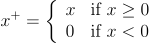
The plus function is defined by

x^+ =<br /> \left\{<br /> \begin{array}{ll}<br /> x & \mbox{if } x \geq 0 \\<br /> 0 & \mbox{if } x < 0 \end{array} \right.

In machine learning the plus is called ReLU (rectified linear unit) but x+ is conventional mathematical notation.

The softplus function approximates x+ by

\text{softplus}(x) = \log(1 + \exp(x))

We can add a parameter to the softplus function to control how soft it is.

\text{softplus}(x; k) = \frac{1}{k}\log\left(1 + \exp(kx)\right)

As the parameter k increases, softmax becomes “harder.” It more closely approximates x+ but at the cost of the derivative at 0 getting larger.

We won’t need other “soft” functions for the rest of the post, but I’ll mention a couple more while we’re here. Softmax is a smooth approximation to the max function

\text{softmax}(x, y) = \log\left(\exp(x) + \exp(y)\right)

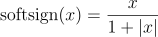
and softsign is a smooth approximation to the sign function.

\text{softsign}(x) = \frac{x}{1 + |x|}

which is differentiable at the origin, despite the absolute value in the denominator. We could add a sharpness parameter k to the softmax and softsign functions like we did above.

Sigmoid

The sigmoid function, a.k.a. the logistic curve, is defined by

\sigma(x) = \frac{\exp(x)}{1 + \exp(x)} = \frac{1}{1 + \exp(-x)}

The second and third expressions are clearly equal, but I prefer to think in terms of the former, but the latter is better for numerical calculation because it won’t overflow for large x.

The sigmoid function is the derivative of the softplus function. We could define a sigmoid function with a sharpness parameter k by taking the derivative of the softplus function with sharpness parameter k.

Swish

The Swish function was defined in [1] as

\text{swish}(x) = x \, \sigma(x)

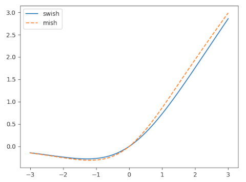
Like softplus, the Swish function is asymptotically 0 as x → −∞ and asymptotically equal to x as x → ∞. That is, for large |x|, swish(x) is approximately x+. However, unlike softplus, swish(x) is not monotone. It is negative for negative x, having a minimum around -1.278 [2]. The fact that the activation function can dip into negative territory is what addresses “the dying ReLU problem,”

Mish

The Mish function was defined in [3] as

\text{mish}(x) = x \, \tanh(\,\text{softplus}(x)\,)

The mish function has a lot in common with the swish function, but performs better, at least on the examples the author presents.

The mish function is said to be part of the swish function family, as is the serf function below.

Serf

The serf function [4] is another variation on the swish function with similar advantages.

\text{serf}(x) = x \, \text{erf}(\,\text{softplus}(x)\,)

The name “serf” comes from “log-Softplus ERror activation Function” but I’d rather pronounce it “zerf” from “x erf” at the beginning of the definition.

The serf function is hard to distinguish visually from the mish function; I left it out of the plot above to keep the plot from being cluttered. Despite the serf and mish functions being close together, the authors in [4] says the former outperforms the latter on some problems.

Numerical evaluation

The most direct implementations of the softplus function can overflow, especially when implemented in low-precision floating point such as 16-bit floats. This means that the mish and serf functions could also overflow.

For large x, exp(x) could overflow, and so computing softplus as

   log(1 + exp(x))

could overflow while the exact value would be well within the range of representable numbers. A simple way to fix this would be to have the softmax function return x when x is so large that exp(x) would overflow.

As mentioned above, the expression for the sigmoid function with exp(-x) in the denominator is better for numerical work than the version with exp(x) in the numerator.

Related posts

[1] Swish: A Self-Gated Activation Function. Prajit Ramachandran∗, Barret Zoph, Quoc V. arXiv:1710.05941v1

[2] Exact form of the minimum location and value in terms of the Lambert W function discussed in the next post.

[3] Mish: A Self Regularized Non-Monotonic Activation Function. Diganta Misra. arXiv:1908.08681v3

[4] SERF: Towards better training of deep neural networks using log-Softplus ERror activation Function. Sayan Nag, Mayukh Bhattacharyya. arXiv:2108.09598v3

Named entity recognition

Named entity recognition (NER) is a task of natural language processing: pull out named things text. It sounds like trivial at first. Just create a giant list of named things and compare against that.

But suppose, for example, University of Texas is on your list. If Texas is also on your list, do you report that you have a named entity inside a named entity? And how do you handle The University of Texas? Do you put it on your list as well? What about UT? Can you tell from context whether UT stands for University of Texas, University of Toronto, or the state of Utah?

Searching for Rice University would be even more fun. The original name of the school was The William Marsh Rice Institute for the Advancement of Letters, Science, and Art. I don’t know whether the name was ever officially changed. A friend who went to Rice told me they had a ridiculous cheer that spelled out every letter in the full name. And of course rice could refer to a grain.

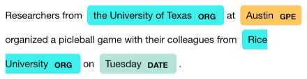
Let’s see what happens when we run the following sentence through spaCy looking for named entities.

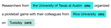
Researchers from the University of Texas at Austin organized a picleball game with their colleagues from Rice University on Tuesday.

I deliberately did not capitalize the definite article in front of University of Texas because I suspected spaCy might include the article if it were capitalized but not otherwise. It included the article in either case.

The results depend on the language model used. When I used en_core_web_trf it included at Austin as part of the university name.

When I used the smaller en_core_web_sm model it pulled out Austin as a separate entity.

The tag ORG stands for organization and DATE obviously stands for date. GPE is a little less obvious, standing for geopolitical entity.

When I changed Rice University to simply Rice, spaCy still recognized Rice as an organization. When I changed it to rice with no capitalization, it did not recognize it as an organization.

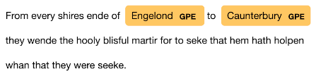
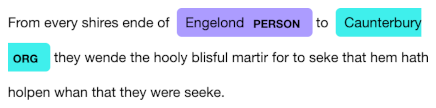
The other day I stress tested spaCy by giving it some text from Chaucer’s Canterbury Tales. Even though spaCy is trained on Modern English, it did better than I would have expected on Middle English.

Using the en_core_web_trf model it recognizes Engelond and Caunterbury as cities.

When I switched to  en_core_web_sm it still recognized Caunterbury as city, but tagged Engelond as a person.


Trying NLP on Middle English

It’s not fair to evaluate NLP software on a language it wasn’t designed to process, but I wanted to try it anyway.

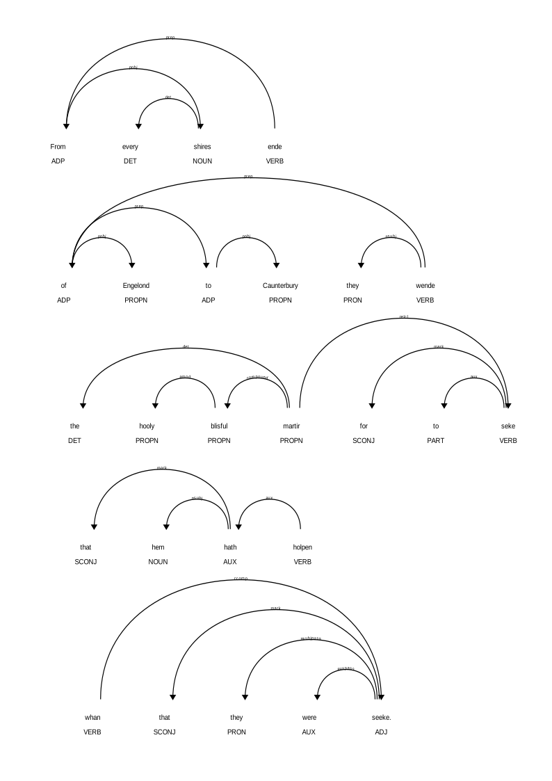
The models in the spaCy software library were trained on modern English text and not on Middle English. Nevertheless, spaCy does a pretty good job of parsing Chaucer’s Canterbury Tales, written over 600 years ago. I used the model en_core_web_lg in my little experiment below.

The text I used comes from the prologue:

From every shires ende
of Engelond to Caunterbury they wende
the hooly blisful martir for to seke
that hem hath holpen
whan that they were seeke.

The software correctly identifies, for example, wende (went) and seke (seak) as verbs, and seeke (sick) as an adjective. Overall it does a pretty good job. I imagine it would do worse on Middle English text that differed more from Modern English usage, but so would a contemporary human who doesn’t know Middle English.

Related posts

How an LLM might leak medical data

Machine learning models occasionally memorize training data. Under the right prompt, a model could return portions of the training data verbatim.

If a large language model is trained on deidentified medical data, along with data that overlaps with the medical data, it could potentially leak details of a person’s medical history. I’m not saying that any particular LLM does leak data, but it’s something to watch out for if you are training an LLM.

One way to try to create a data leak would be to prompt the LLM with the data you have and see whether it will fill in more. For example, I asked Bing AI

Tell me about a man from Arkansas with ICD-10 code C50.921.

It came back with the following.

… Once upon a time, there was a man named John who lived in Arkansas. John was a hardworking man who loved spending time with his family and friends. One day, John noticed a lump in his right breast. He went to the doctor and was diagnosed with malignant neoplasm of unspecified site of the right male breast, classified under the ICD-10 code C50.921. …

I chose this diagnosis code because male breast cancer is extremely rare, and so the risk of reidentification is higher than for a more common diagnosis.

The model filled in the detail that the man’s name is John. This is not at all suspicious since John is the one of the most common male names in history. If the man’s name had been Vivek, there would be more cause to suspect the model is telling us about a real man name Vivek, though of course that could be a randomly chosen male name.

If a neural network were training on deidentified medical data, it could link fields together. If the story above had said “John, aged 42, …” the age might have been pulled from an actual patient record.

If the data the network was trained on was deidentified well, even leaking data verbatim should not create more than a very small risk of identification. However, if the data contained tokens linking the records to publicly available information, such as real estate records—this happens—then our hypothetical LLM might reveal more personal details that could be used to narrow down whose data is being leaked.

Related posts

Experiments with Bing chat

My two previous posts looked at experiments with ChatGPT and Google Bard. This post will look at redoing the same experiments with Microsoft’s Bing Chat: looking for mnemonic encodings and simplifying Boolean expressions.

When you open up Bing chat you can select a conversational style:

  • More creative
  • More balanced
  • More precise

I chose “more precise” for my experiments.

Mnemonic encodings

Bing seems to “know” more about the Major mnemonic system. In response to my first question about the system it gave a link to the Wikipedia article on the Major system and a couple other relevant links. It gives a more complete table of encodings than ChatGPT did:

  • 0: s, z
  • 1: t, d, th
  • 2: n
  • 3: m
  • 4: r
  • 5: l
  • 6: j, ch, sh
  • 7: c, k, g, q, ck
  • 8: v, f, ph
  • 9: p, b

Directly asking for encodings

It seems to do pretty well when I ask for an encoding of a two-digit number, and when I ask for an encoding of a three-digit number it encodes the first two digits correctly but ignores the third digit. However, when I asked it to encode 345 it did very well:

Using the Major System, the number 345 can be encoded as “molar” or “mailer” or “miller” or “mural” or “marl”, among others.

ChatGPT and Google Bard said that no English word can encode 345, though Google Bard came up with Merlin anyway. (Strictly speaking “Merlin” encodes 3452, but it’s a common practice to just pay attention the first three consonants in words with more than three consonants.)

Asking for sounds

When I asked “Find a word with the sounds g, r, and f” Bing came back with

 One word that contains the sounds g, r, and f is “giraffe” 🦒

When I asked for the sounds l, f, and b, Bard came up with “belief.” When I added “in that order” to my prompt it came back with “bluff” and “flyby,” ignoring the order requirement.

In general Bing AI seems to do better that ChatGPT and Bard at word game questions.

Boolean minimization

Next I tried the Boolean minimization problem that I’d tried with ChatGPT and Bard using the prompt

Minimize the boolean expression ¬AB¬C¬D + A¬B¬C¬D + A¬B¬CD + A¬BC¬D + A¬BCD + AB¬C¬D + ABC¬D + ABCD

ChatGPT tried a Karnaugh map approach, but botched it. Bard tried an algebraic approach, but also botched it.

Bing tried something different:

The given boolean expression can be simplified using the consensus theorem. The consensus theorem states that for any three variables A, B, and C: AB + AC + BC = AB + AC. Applying this theorem to the given expression, we get

¬AB¬C¬D + A¬B¬C¬D + A¬B¬CD + A¬BC¬D + A¬BCD + AB¬C¬D + ABC¬D + ABCD
= ¬AB¬C¬D + A¬B¬C¬D + A¬B¬CD + A¬BC¬D + A¬BCD + AB¬C¬D + ABC
= ¬AB¬C¬D + A( ¬B¬C¬D + ¬B¬CD + ¬BC¬D + ¬BCD) + AB( ¬C¬D) + ABC
= ¬AB( ¬C) ( ¬D) + A( ¬B) ( ¬C( ¬D) + ¬CD) + AB( ¬C( ¬D)) + ABC
= ¬AB( ¬C) ( ¬D) + A( ¬B) ( ¬CD) + AB( ¬C( ¬D)) + ABC
= (A+B)(A+C)(A+D)(B+C)(B+D)(C+D)

This derivation starts out correctly but goes astray about halfway through.