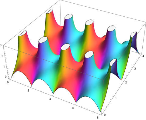
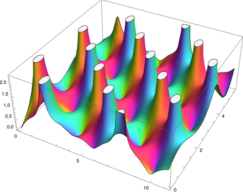
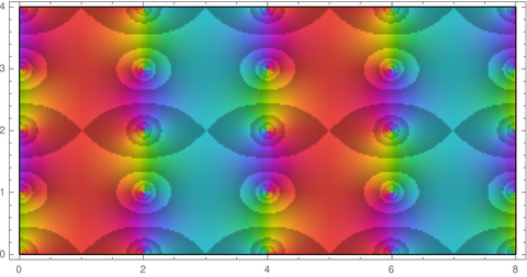
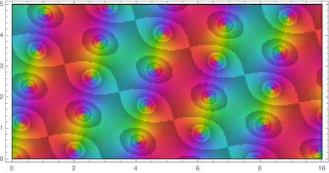
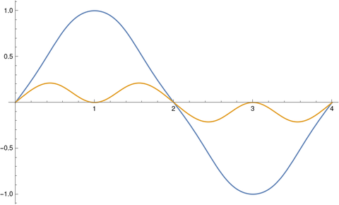
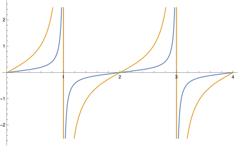
As discussed in the previous post, the Jacobi elliptic function sn(z, m) is doubly periodic in the complex plane, with period 4K(m) in the horizontal direction and period 2K(1-m) in the vertical direction. Here K is the complete elliptic integral of the first kind.
The function sn(z, m) maps the rectangle
(−K(m), K(m)) × (0, K(1−m))
conformally onto to the upper half plane, i.e. points in the complex plane with non-negative imaginary part.
For example, sn(z, 0.5) takes the rectangle
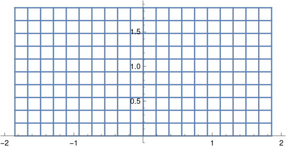
to
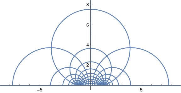
The function sn has a singularity at the top middle of the rectangle, and so as horizontal lines approach the top of the rectangle, their image turns into bigger and bigger circles. filling the half plane.
The plot above was created with the following Mathematica code:
    K = EllipticK[1/2]
    Show[
        ParametricPlot[
            Table[{Re[JacobiSN[x + I y, 0.5]], Im[JacobiSN[x + I y, 0.5]]},
            {x, -K, K, K/10}], {y, 0, K}],
        ParametricPlot[
             Table[{Re[JacobiSN[x + I y, 0.5]], Im[JacobiSN[x + I y, 0.5]]},
             {y, 0, K, K/10}], {x, -K, K}],
        PlotRange -> {{-8, 8}, {0, 8}}]
You can vary the parameter m to match the shape of the rectangle you want to map to the half plane. You cannot choose both the length and width of your rectangle with only one parameter, but you can choose the aspect ratio. By choosing m = 1/2 we got a rectangle twice as wide as it is tall.
In our example we have a rectangle 3.70815 wide and 1.85407 tall. If we wanted a different size but the same aspect ratio, we could scale the argument to sn. For example,
sn(Kz, 0.5)
would map the rectangle (−1, 1) × (0, 1) onto the open half plane where K is given in the Mathematica code above.
In general we can solve for the parameter m that gives us the desired aspect ratio, as explained in the previous post, then find k such that sn(kz, m) maps the rectangle of the size we want into the half plane.
The inverse function, mapping the half plane to the rectangle, can be found in terms of elliptic integrals. Mathematica provides a convenient function InverseJacobiSN for this.
We could map any rectangle conformally to any other rectangle by mapping the first rectangle to the upper half plane, then mapping the upper half plane to the second rectangle. (We can’t simply scale the rectangle directly because such a map will not be conformal, will not preserve angles, unless we scale horizontally and vertically by the same amount. We can find a conformal map that will change the aspect ratio of a rectangle, but it will not simply scale the rectangle linearly.)
Although we can conformally map between any two rectangles using the process described above, we may not want to do things this way; the result may not be what we expect. Conformal maps between regions are not quite unique. They are unique if you specify where one point in the domain goes and specify the argument of its derivative. You may need to play with those extra degrees of freedom to get a conformal map that behaves as you expect.
Related posts