Halley’s variation on Newton’s method

Newton’s method for solving f(x) = 0 converges quickly once it starts to converge. Specifically, it converges quadratically: the error is roughly squared at each step. This means that the number of correct decimal places doubles at each iteration of Newton’s method.

Doubling the number of decimal places is nice, but what if we could triple the number of correct decimals at each step? Edmond Halley, best known for the comet that bears his name, came up with a way to do just that. Newton’s method converges quadratically, but Halley’s method converges cubically.

Newton’s method updates iterations using the rule

x_{n+1} = x_n + \frac{f(x_n)}{f'(x_n)}

Halley’s variation uses the rule

x_{n+1} = x_n - \frac{1}{\dfrac{f'(x_n)}{f(x_n)} - \dfrac{f''(x)}{2f'(x)}}

Halley’s method makes more progress per iteration, but it also takes more work per iteration, and so in practice it’s not usually an improvement over Newton’s method. But in some cases it could be.

Evaluating efficiency

In root-finding problems, the function f is usually relatively time-consuming to evaluate. We can assume nearly all the work in root-finding goes into evaluating f and its derivatives, and we can ignore the rest of the arithmetic in the method.

Newton’s method requires evaluating the function f and its derivative f ′. Halley’s method requires these function evaluates as well and also requires evaluating the second derivative f ′′.

Three iterations of Newton’s method make as much progress toward finding a root as two iterations of Halley’s method. But since Newton’s method requires two function evaluations and Halley’s method requires three, both require six function evaluations to make the same amount of progress. So in general Halley’s method is not an improvement over Newton’s method.

When Halley might be better

Suppose we had a way to quickly compute the second derivative of f at a point from the values of f and its first derivative at that point, rather than by having to evaluate the second derivative explicitly. In that case two iterations of Halley’s method might make as much progress as three iterations of Newton’s method but with less effort, four function evaluations rather than six.

Many of the functions that are used most in applied mathematics satisfy 2nd order differential equations, and so it is common to be able to compute the second derivative from the function and its derivative.

For example, suppose we want to find the zeros of Bessel functions Jν. Bessel functions satisfy Bessel’s differential equation; that’s where Bessel functions get their name.

x^2 y'' + x y' + \left(x^2 - \nu^2 \right) y = 0

This means that once we have evaluated Jν and its first derivative, we can compute the second derivative from these values as follows.

J_{\nu}''(x_n) = \frac{(\nu^2 - x_n^2)J_\nu(x_n) - x_nJ_\nu'(x_n)}{x_n^2}

Maybe we’re not working with a well-studied function like a Bessel function but rather we are numerically solving a differential equation of our own creation and we want to know where the solution is zero. Halley’s method would be a natural fit because our numerical method will give us the values of y and y ′ at each step.

Related posts

Drag equation exponent variation

The motion of a falling body of mass m is given by

m \frac{dv}{dt} = mg - kv^r

where the term −kvr accounts for drag due to air resistance. One can derive r = 2 under simple physical assumptions, but if I remember correctly other values of r may be more realistic in certain circumstances. I don’t know much about the physics here; if you know about the use of other values of r, please let me know by leaving a comment.

Terminal velocity

When r = 1 or r = 2 the differential equation above can be solved in terms of elementary functions, but otherwise it cannot. Nevertheless one can show that for all values of r the object reaches a terminal velocity, and calculate that velocity without explicitly solving the differential equation. William Waterhouse demonstrated this in a one-page article [1]. He rewrites the equation to look at time as a function of velocity rather than velocity as a function of time

\frac{dt}{dv} = \frac{1}{g} \frac{1}{1 - (k/mg)v^r}

and concludes

t = \frac{1}{g} \int_0^v \frac{dv}{1 - (k/mg)v^r} + t_0

He notes that the integral diverges as v approaches

 \left(\frac{mg}{k}\right)^{1/r}

and so that is the terminal velocity, i.e. it takes an infinite amount of time to achieve this velocity. Waterhouse recommends this derivation as “a good example of deriving information about a problem without knowing an explicit solution.”

I would add that such an approach is the norm, not an exception. A closed-form solution to a differential equation in nice when you can get it, but usually not possible. And even when you can find a closed-form solution, you may be able to achieve your goal more directly by not using it.

Hypergeometric solution

I suspected the differential equation could be solved for general values of r using special functions, and that is the case. Mathematica was able to evaluate the integral for t as a function of v in terms of a hypergeometric function.

v \, _2F_1\left(1,\frac{1}{r};1+\frac{1}{r};\frac{g k v^r}{m}\right)

When I asked Mathematica to solve the differential equation directly, it said that the solution is the inverse function of the function above. Apparently Waterhouse and Mathematica agree that it is easier to think of t as a function of v rather than the original formulation.

The notation 2F1 indicates there are two upper parameters and one lower parameter. In our application, the upper parameters are 1 and 1/r, the lower parameter is 1 + 1/r, and the function is evaluated at gkvr/m. You can find a brief introduction to hypergeometric functions here. A hypergeometric function 2F1 has a singularity at 1, and so we could derive the terminal velocity from the explicit solution.

Mathematica implementation

Let c = gk/m. Then we can express velocity as a function of time in Mathematica by

    f[r_, c_, v_] := InverseFunction
    [
        #1 Hypergeometric2F1[1, 1/r, 1 + 1/r, c #1^r] &
    ][t]

and use this to make plots of the velocity for various values of c and r.

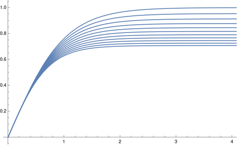
The following sets c = 2 and varies r over 1, 1.1, 1.2, … 2.

    Plot[Table[f[2, d/10, t], {d, 10, 20}], {t, 0, 4}, PlotRange -> All]

Here’s the output.

The terminal velocity decreases as r increases. The opposite is true for c < 1.

[1] William C. Waterhouse. A Fact about Falling Bodies. Mathematics Magazine, Vol. 44, No. 1 (Jan., 1971), pp. 33–34. The article straddles two pages, but takes up less than half of each page.

Moving between differential and integral equations

My years in graduate school instilled a Pavlovian response to PDEs: multiply by a test function and integrate by parts. This turns a differential equation into an integral equation [1].

I’ve been reading a book [2] on integral equations right now, and it includes several well-known techniques for turning certain kinds of integral equations into differential equations. Then this afternoon I talked to someone who was excited to have discovered a way to turn a more difficult integral equation into a differential equation.

For theoretical purposes, you often want to turn differential equations into integral equations. But for computational purposes, you often want to do the reverse.

Differential and integral equations are huge, overlapping fields, and sweeping generalities have exceptions. The opposite of the statement above may also be true. You may want to turn a differential equation into an integral equation for computational purposes (as in the finite element method) or turn an integral equation into a differential equation for theoretical convenience (as was the case for the person I was taking to).

***

[1] Sorta. More precisely this moves from the strong form of the PDE to a weak form. This involves integration, at least formally.

[2] Vladimir Ryzhov et al. Modern Methods in Mathematical Physics: Integral Equations in Wolfram Mathematica.

The essence of chaos

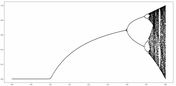
logistic bifurcation diagram

Linear systems can show sensitive dependence on initial conditions, but they cannot be chaotic. Only nonlinear systems can be chaotic.

George Datseris and Ulrich Parlitz explain this well in their book Nonlinear Dynamics:

… Sensitive dependence is not sufficient for a definition of chaos. … the state space is first stretched and then folded within itself. This is the defining characteristic of chaotic systems. The stretching part is where sensitive dependence comes from … as state space volumes increase in size … nonlinear dynamics takes over and folds the state space back in on itself. … This is why only nonlinear systems can be chaotic: linear systems with positive Lyapunov exponents always escape to infinity.

Related posts

The Pearson distributions

The previous post was about 12 probability distributions named after Irving Burr. This post is about 12 probability distributions named after Karl Pearson. The Pearson distributions are better known, and include some very well known distributions.

Burr’s distributions are defined by their CDFs; Pearson’s distributions are defined by their PDFs.

Pearson’s differential equation

The densities of Pearson’s distributions all satisfy the same differential equation:

f'(x) = \frac{(x-a) f(x)}{c_0 + c_1x + c_2x^2}

This is a linear differential equation, and so multiples of a solution are also a solution. However, a probability density must integrate to 1, so there is a unique probability density solution given a, c0, c1, and c2.

Well known distributions

Note that f(x) = exp(-x²/2) satisfies the differential equation above if we set a = 0, c0 = 1, and c1 = c2 = 0. This says the normal distribution is a Pearson distribution.

If f(x) = xm exp(-x) then the differential equation is satisfied for am, c0 = −1, and c0 = c2 = 0. This says that the exponential distribution and more generally the gamma distribution are Pearson distributions.

You can also show that the Cauchy distribution and more generally the Student t distribution are also Pearson distributions. So are the beta distributions (with a transformed range).

Table of Pearson distributions

The table below lists all Pearson distributions with their traditional names. The order of the list is a little strange for historical reasons.

The table uses Iverson’s bracket notation: a Boolean expression in brackets represents the function that is 1 when the condition holds and 0 otherwise. This way all densities are defined over the entire real line, though some of them are only positive over an interval.

The densities are presented without normalization constant; the normalization constant are whatever they have to be for the function to integrate to 1. The normalization constants can be complicated functions of the parameters and so they are left out for simplicity.

\begin{align*} \text{I} \hspace{1cm} & (1+x)^{m_1} (1-x)^{m_2} \,\,[-1 \leq x \leq 1] \\ \text{II} \hspace{1cm} & (1 - x^2)^m \,\, [ -1 \leq x \leq 1] \\ \text{III} \hspace{1cm} & x^m \exp(-x) \,\, [0 \leq x] \\ \text{IV} \hspace{1cm} & (1 + x^2)^{-m} \exp(-v \arctan x) \\ \text{V} \hspace{1cm} & x^{-m} \exp(-1/x) \,\, [0 \leq x] \\ \text{VI} \hspace{1cm} & x^{m_2}(1 + x)^{-m_1} \,\,[0 \leq x] \\ \text{VII} \hspace{1cm} & (1 + x^2)^{-m}\\ \text{VIII} \hspace{1cm} & (1 + x)^{-m} \,\, [0 \leq x \leq 1] \\ \text{IX} \hspace{1cm} & (1 + x)^{m} \,\, [0 \leq x \leq 1] \\ \text{X} \hspace{1cm} & \exp(-x) \,\, [0 \leq x] \\ \text{XI} \hspace{1cm} & x^{-m} \,\,[1 \leq x] \\ \text{XII} \hspace{1cm} & \left( (g+x)(g-x)\right)^h \,\, [-g \leq x \leq g] \end{align*}

There is a lot of redundancy in the list. All the distributions are either special cases of or limiting cases of distributions I, IV, and VI.

Note that VII is the Student t distribution after you introduce a scaling factor.

Moments

The Pearson distributions are determined by their first few moments, provided these exist, and these moments can be derived from the parameters in Pearson’s differential equation.

This suggests moment matching as a way to fit Pearson distributions to data: solve for the distribution parameters that make the the exact moments match the empirical moments. Sometimes this works very well, though sometimes other approaches are better, depending on your criteria for what constitutes a good match.

Heat equation and the normal distribution

The density function of a normal distribution with mean 0 and standard deviation √(2kt) satisfies the heat equation. That is, the function

u(x, t) = \frac{1}{2\sqrt{\pi kt}} \exp\left(-\frac{x^2}{4kt}\right)

satisfies the partial differential equation

u_t = k\,u_{xx}

You could verify this by hand, or if you’d like, here’s Mathematica code to do it.

      u[x_, t_] := PDF[NormalDistribution[0, Sqrt[2 k t]], x]
      Simplify[ D[u[x, t], {t, 1}] - k D[u[x, t], {x, 2}] ]

This returns 0 as expected.

Solutions to the heat equation are unique if we specify initial conditions. So if we start with a very concentrated heat source at time t = ε, say

u(x, \varepsilon) = \frac{1}{2\sqrt{\pi k\varepsilon}} \exp\left(-\frac{x^2}{4k\varepsilon}\right)

where ε is a tiny but positive number, then the solution at the top of the post hold for all t > 0 and is unique.

Alternatively, we could say that if our initial condition is u(x, 0) = δ where the right hand side is the Dirac delta function, then the solution at the top of the post holds for all t > 0 and is unique. You could justify this rigorously using distribution theory (in the analytic sense, not the probability sense, though they’re related). Or you could justify it heuristically by letting ε to go zero and thinking of δ as the limit.

It is also the case that a constant satisfies the heat equation. So if we add a constant to our solution, the constant representing ambient temperature, and add our initial condition to that constant, the solution is the constant plus the solution above.

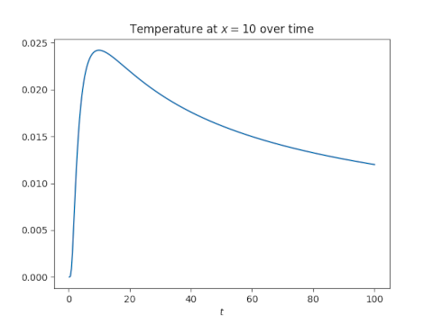
The temperature at the center will decay in proportion to 1/√t. A point x away from the center will initially get warmer, reach a maximum temperature at time t = x²/2k, and then cool off roughly in proportion to 1/√t.

Here’s a plot of the temperature at x = 10 with k = 5.

Related posts

Third order ordinary differential equations

Most applied differential equations are second order. This probably has something to do with the fact that Newton’s laws are second order differential equations.

Higher order equations are less common in application, and when they do pop up they usually have even order, such as the 4th order beam equation.

What about 3rd order equations? Third order equations are rare in application, and third order linear equations are even more rare.

This post will focus on ordinary differential equations (ODEs), but similar remarks apply to PDEs.

Third order nonlinear equations

One example of a third order nonlinear ODE is the Blasius boundary layer equation from fluid dynamics

y''' + yy'' = 0

and its generalization, the Falkner-Skan equation

y''' + yy'' + \beta\left(1 - (y')^2\right) = 0.

Third order linear equations

I’ve seen two linear third order ODEs in application, but neither one is very physical.

The first [1] is an equation satisfied by the product of Airy functions:

 y''' - 4xy' - 2y = 0.

Here is a short proof that the product of Airy functions satisfy this equation.

Airy functions come up in applications such as quantum mechanics, optics, and probability. I suppose products of Airy functions may come up in those areas, but the equation above seems like something discovered after the fact. It seems someone thought it would be useful to find a differential equation that products of Air functions satisfy. I doubt someone wrote down the equation because it came up in applications, then discovered that products of Airy functions were the solutions.

The second [2] is a statistical model for analyzing handwriting:

x'''(t) = \beta_1(t) x'(t) + \beta_2(t) x''(t) + f(t).

Here someone decided to try modeling handwriting movements as a function of velocity, acceleration, and “jerk” (third derivative of position). It may be a useful model, but it wasn’t derived in the same physical sense as say the equations of mechanical vibrations. You could also object that since x(t) does not appear in the equation, this is a second order differential equation for y(t) = x′(t).

Related posts

[1] Abramowitz and Stegun, Handbook of Mathematical Functions, equation 10.4.57.

[2] Ransay and Silverman. Applied Functional Data Analysis: Methods and Case Studies. Equation 12.1.

Finding a vector potential whose curl is given

The previous post showed that if a vector field F over a simply connected domain has zero curl, then there is a potential function φ whose gradient is F.

An analogous result says that if the vector field F has zero divergence, again over a simply connected domain, then there is a vector potential Φ whose curl is F.

These are both special cases of Poincaré’s lemma.

This post will outline how to calculate Φ. First of all, Φ is far from unique. Any vector field with zero curl can be added to Φ without changing its curl. So if

Φ = (Φ1, Φ2, Φ3)

then we can assume that one of the components, say Φ3, is zero by adding the right curl-free component. If you find that argument less than convincing, look at it this way: we’re going to solve a harder problem than simply find Φ such that ∇×Φ = F by giving ourselves the additional requirement that the last component of Φ must be zero.

Now if Φ = (Φ1, Φ2, 0) and ∇×Φ = F, then

−∂z Φ2= F1
z Φ1 = F2
x Φ2 − ∂y Φ1 = F3

We can solve the first equation by integrating F1 with respect to z and adding a function of x and y to be determined later. We can solve the second equation similarly, then use the third equation to determine the functions of x and y left over from solving the first two equations.

***

This post is the third, and probably last, in a series of posts looking at vector calculus from a more advanced perspective.  The first post in the series looked at applying {grad, curl, div} to {grad, curl, div}: seeing which combinations are defined, and which combinations are always 0. To illustrate the general pattern, the post dips into differential forms and the Hodge star operator.

The second post looked at finding the (scalar) potential function for a curl-free vector field, and mentions connections to topology and differential equations.

The present post is a little terse, but it makes more sense if you’ve gone through the previous post. The method of solution here is analogous to the method in the previous post, and that post goes into a little more detail.

Conservative vector fields

The previous post discussed the fact that the curl of a divergence is zero. The converse is also true (given one more requirement): a vector field F is the gradient of some potential φ function if ∇×F = 0. In that case we say F is a conservative vector field.

It’s clear that having zero curl is a necessary condition for a vector field to be the gradient of a potential. It’s not as clear that having zero curl is sufficient. And in fact, it’s not quite sufficient: it’s sufficient over a simply connected domain. This means a domain with no holes: any loop you draw in the domain can be continuously deformed to a point without leaving the domain. If you’re working with vector fields defined everywhere on ℝ³ then you don’t have to worry about this condition because ℝ³ is simply connected.

Aside on topology

For a calculus student, the requirement that a domain be simply connected is a footnote. For a topologist, it’s the main thing.

If a domain is not simply connected, then a vector field might have curl zero, but not be the gradient of a potential. So in general we have two kinds of vector fields with zero curl: those that are gradients and those that are not. We could look at the space of all vector fields that have zero curl and mod out by the vector fields that are gradients. The dimension of this space tells us something about how the domain is connected. This is the start of de Rham cohomology.

Calculating the potential function

If a vector field is conservative, i.e. if it is the gradient of a potential function φ, then you can find φ by integration.

The partial derivative of φ with respect to x is the first component of your vector field, so you can integrate to find φ as a function of x (and y and z). This integral will only be unique up to a constant, and functions of y and z alone are constants as far as partial derivatives with respect to x are concerned.

Now the partial derivative of φ with respect to y has to equal the second component of your vector field. So taking the derivative of what you found above determines your potential, up to a function of z. So then you differentiate again, this time with respect to z, and set this equal to the third component of your vector field, you’ve determined your potential function up to an constant. And that’s as far as it can be determined: any constant term goes away when you take the gradient.

Exact differential equations

A differential equation of the form

M(x, y) + N(x, y) y‘(x) = 0

is said to be exact if the partial derivative of M with respect to y equals the partial of N with respect to x. In that case you can find a function φ such that the partial of φ with respect to x is M and the partial of φ with respect to y is N (assuming you’re working in a simply connected domain). This function φ is a potential, though differential equation texts don’t call it that, and you find it just as you found φ above. The solution to your differential equation is given (implicitly) by

φ(x, y) = c

where c is a constant to be determined by initial conditions.

Poincaré’s lemma

For a vector field over a simply connected domain, having zero curl is necessary and sufficient for the existence of a potential function φ. This is a case of Poincaré’s lemma. The next post will look at another case of Poincaré’s lemma, finding a vector potential.

Solving Laplace’s equation in the upper half plane

In the previous post, I said that solving Laplace’s equation on the unit disk was important because the unit disk is a sort of “hub” of conformal maps: there are references and algorithms for mapping regions to and from a disk conformally.

The upper half plane is a sort of secondary hub. You may want to map two regions to and from each other via a half plane. And as with the disk, there’s an explicit solution to Laplace’s equation on a half plane.

Another reason to be interested in Laplace’s equation on a half plane is the connection to the Hilbert transform and harmonic conjugates.

Given a continuous real-valued function u on the real line, u can be extended to a harmonic function on the upper half plane by taking the convolution of u with the Poisson kernel, a variation on the Poisson kernel from the previous post. That is, for y > 0,

u(x + iy) = \frac{1}{\pi} \int_{-\infty}^\infty \frac{y}{(x-t)^2 + y^2}\, u(t)\, dt

This gives a solution to Laplace’s equation on the upper half plane with boundary values given by u on the real line. The function u is smooth on the upper half plane, and its limiting values as y → 0 is continuous.

Furthermore, u is the real part of an analytic function f = u + iv. The function v is the harmonic conjugate of u, and also equals the Hilbert transform of u.