Three surprises with the trapezoid rule

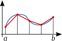
The trapezoid rule is a very simple method for estimating integrals. The idea is to approximate the area under a curve by a bunch of thin trapezoids and add up the areas of the trapezoids as suggested in the image below.

This is an old idea, probably older than the formal definition of an integral. In general it gives a crude estimation of the integral. If the width of the trapezoids is h, the error in using the trapezoid rule is roughly proportional to h2. It’s easier to do better. For example, Simpson’s rule is a minor variation on the trapezoid rule that has error proportional to h5.

So if the trapezoid rule is old and inaccurate, why does anyone care about it? Here are the surprises.

The last two observations are more widely applicable than you might think at first. What if you want to integrate something that isn’t periodic and isn’t a double exponential function? You may be able to do a change of variables that makes your integrand have one of these special forms. The article Fast Numerical Integration explains an integration method based on double exponential functions and includes C++ source code.

The potential efficiency of the trapezoid rule illustrates a general principle: a crude method cleverly applied can beat a clever technique crudely applied. The simplest numerical integration technique, one commonly taught in freshman calculus, can be extraordinarily efficient when applied with skill to the right problem. Conversely, a more sophisticated integration technique such as Gauss quadrature can fail miserably when naively applied.

Related posts

Optical illusion, mathematical illusion

Someone sent me a link to an optical illusion while I was working on a math problem. The two things turned out to be related.

In the image below, what look like blues spiral and green spirals are actually exactly the same color. The spiral that looks blue is actually green inside, but the magenta stripes across it make the green look blue. I know you don’t believe me; I didn’t believe it either. You can open it in an image editor and use a color selector to examine it for yourself.

My math problem was also a case of two things that look different even though they are not. Maybe you can think back to a time as a student when you knew your answer was correct even though it didn’t match the answer in the back of the book. The two answers were equivalent but written differently. In an algebra class you might answer 5 / √3 when the book has 5 √3 / 3. In trig class you might answer 1 − cos2 x when the book has sin2 x. In a differential equations class, equivalent answers may look very different since arbitrary constants can obfuscate differences.

In my particular problem, I was looking at weights for Gauss-Hermite integration. I was trying to reconcile two different expressions for the weights, one in some software I’d written years ago and one given in Abramowitz and Stegun. I thought I’d found a bug, at least in my comments if not in my software. My confusion was analogous to not recognizing a trig identity.  I wish I could say that the optical illusion link made me think that the two expressions may be the same and they just look different because of a mathematical illusion. That would make a good story. Instead, I discovered the equivalence of the two expressions by brute force, having Mathematica print out the values so I could compare them. Only later did I see the analogy between my problem and the optical illusion.

In case you’re interested in the details, my problem boiled down to the equivalence between Hn+1(xi)2 and 4n2Hn−1(xi)2 where Hn(x) is the nth Hermite polynomial and xi is the ith root of Hn. Here’s why these are the same. The Hermite polynomials satisfy a recurrence relation

Hn+1(x) = 2x Hn(x) − 2n Hn−1(x)

for all x. Since Hn(xi) = 0, Hn+1(xi) = −2nHn−1(x). Now square both sides.

Related post: Orthogonal polynomials

Quasi-random sequences in art and integration

Sometimes when people say they want random points, that’s not what they really want. Random points clump more than most people expect. Quasi-random sequences are not random in any mathematical sense, but they might match popular expectations of randomness better than the real thing, especially for aesthetic applications. If by “random” someone means “scattered around without a clear pattern and not clumped together” then quasi-random sequences might do the trick.

Here are the first 50 points in a quasi-random sequence of points in the unit square.

quasi-random points

By contrast, here are 50 points in a unit square whose coordinates are uniform random samples.

random points

The truly random points clump together. Notice the cluster of three points in the top right corner. There are few other instances of pairs of points being very close together. Also, there are fairly large areas that don’t contain any random points. The quasi-random points by contrast are better spread out. They have a self-avoiding property that keeps them from clustering, and they fill the space more efficiently.

Quasi-random sequences could be confused with pseudo-random sequences. They’re not at all the same thing. Pseudo-random sequences are computer-generated sequences that in many ways behave as if they were truly random, even though they were produced by deterministic algorithms. For many practical purposes, including sensitive statistical tests, pseudo-random sequences are simply random sequences. (The “truly” random points above were technically “pseudo-random” points.)

The quasi-random points above were part of a Sobol sequence, a common quasi-random sequence. Other quasi-random sequences include the Halton sequence and the Hammersley sequence. Mathematically, these sequences are defined has having low-discrepancy. Roughly speaking, this means the “discrepancy” between the number of points that actually fall in a volume and the number of points you’d expect to fall in the same volume is small. See the Wikipedia article on quasi-random sequences for more mathematical details.

Besides being aesthetically useful, quasi-random sequences are useful in applied mathematics. Because these sequences explore a space more efficiently than random sequences, quasi-random sequences sometimes lead to more efficient high-dimensional integration algorithms than Monte Carlo integration. Quasi-Monte Carlo integration, i.e. integration based on quasi-random sequences rather than random sequences, is popular in financial applications. Art Owen has written insightful papers on Quasi-Monte Carlo integration (QMC). He has classified which integration problems can be efficiently computed via QMC methods and which cannot. In a nutshell, QMC works well when the effective dimension of a problem is significantly lower than the actual dimension. For example, a financial model might ostensibly depend on 1000 variables, but 50 of those variables contribute far more to the integrand than all the other variables. The integrand might essentially be a function of only 50 variables. In that case, QMC will work well. Note that it is not necessary to identify these 50 variables or do any change of variables. QMC just magically takes advantage of the situation.

One disadvantage of QMC integration is that it doesn’t naturally lead to an estimate of its own accuracy, unlike Monte Carlo integration. Several hybrid approaches have been proposed to combine QMC integration and Monte Carlo integration to get the efficiency of the former and the error estimates of the latter. For example, one could randomly jitter the quasi-random points or randomly permute their components. Some of these results are in Art Owen’s papers.

To read more about quasi-random sequences, see the book Random Number Generation and Quasi-Monte Carlo Methods.

Numerical integration article posted

This weekend CodeProject posted an article I wrote entitled Fast numerical integration.

The algorithm in the article, introduced in the 1970s by Masatake Mori and Hidetosi Takahasi, is indeed fast. It integrates analytical functions over bounded intervals with the most accuracy for a fixed number of integration points.

The CodeProject article includes source code and is mostly about the code. See this page for mathematical details.

Random inequalities III: numerical results

The first post in this series introduced random inequalities. The second post discussed random inequalities can could be computed in closed form. This post considers random inequalities that must be evaluated numerically.

The simplest and most obvious approach to computing P(X > Y) is to generate random samples from X and Y and count how often the sample from X is bigger than the sample from Y. However, this approach is only accurate on average. In any particular sample, the error may be large. Even if you are willing to tolerate, for example, a 5% chance of being outside your error tolerance, the required number of random draws may be large. The more accuracy you need, the worse it gets since your accuracy only improves as n−1/2 where n is the number of samples. For numerical integration methods, the error decreases as a much larger negative power of n depending on the method. In the timing study near the end of this technical report, numerical integration was 2,875 times faster than simulation for determining beta inequality probabilities to just two decimal places. For greater desired accuracy, the advantage of numerical integration would increase.

Why is efficiency important? For some applications it may not be, but often these random inequalities are evaluated in the inner loop of a simulation. A simulation study that takes hours to run may be spending most of its time evaluating random inequalities.

As derived in the previous post, the integral to evaluate is given by

\begin{eqnarray*} P(X \geq Y) &=& \int \!\int _{[x > y]} f_X(x) f_Y(y) \, dy \, dx \\ &=& \int_{-\infty}^\infty \! \int_{-\infty}^x f_X(x) f_Y(y) \, dy \, dx \\ &=& \int_{-\infty}^\infty f_X(x) F_Y(x) \, dx end{eqnarray*}

The technical report Numerical computation of stochastic inequality probabilities gives some general considerations for numerically evaluating random inequalities, but each specific distribution family must be considered individually since each may present unique numerical challenges. The report gives some specific techniques for beta and Weibull distributions.  The report Numerical evaluation of gamma inequalities gives some techniques for gamma distributions.

Numerical integration can be complicated by singularities in integrand for extreme values of distribution parameters. For example, if X ~ beta(a, b) the integral for computing P(X > Y) has a singularity if either a or b are less than 1. For general advice on numerically integrating singular integrands, see “The care and treatment of singularities” in Numerical Methods that Work by Forman S. Acton.

Once you come up with a clever numerical algorithm for evaluating a random inequality, you need to have a way to test the results.

One way to test numerical algorithms for random inequalities is to compare simulation results to integration results. This will find blatant errors, but it may not be as effective in uncovering accuracy problems. It helps to use random parameters for testing.

Another way to test numerical algorithms in this context is to compute both P(X > Y) and P(Y > X). For continuous random variables, these two values should add to 1. Of course such a condition is not sufficient to guarantee accuracy, but it is a simple and effective test. The Inequality Calculator software reports both P(X > Y) and P(Y > X) partly for the convenience of the user but also as a form of quality control: if the two probabilities do not add up to approximately 1, you know something has gone wrong. Along these lines, it’s useful to verify that P(X > Y) = 1/2 if X and Y are identically distributed.

Finally, integrands may have closed-form solutions for special parameters. For example, Exact calculation of beta inequalities gives closed-form results for many special cases of the parameters. As long as the algorithm being tested does not depend on these special values, these special values provide valuable test cases.

Random inequalities II: analytical results

My previous post introduced random inequalities and their application to Bayesian clinical trials. This post will discuss how to evaluate random inequalities analytically. The next post in the series will discuss numerical evaluation when analytical evaluation is not possible.

For independent random variables X and Y, how would you compute P(X>Y), the probability that a sample from X will be larger than a sample from Y? Let fX be the probability density function (PDF) of X and let FX be the cumulative distribution function (CDF) of X. Define fY and FY similarly. Then the probability P(X > Y) is the integral of fX(x) fY(y) over the part of the xy plane below the diagonal line x = y.

\begin{eqnarray*} P(X \geq Y) &=& \int \!\int _{[x > y]} f_X(x) f_Y(y) \, dy \, dx \\ &=& \int_{-\infty}^\infty \! \int_{-\infty}^x f_X(x) f_Y(y) \, dy \, dx \\ &=& \int_{-\infty}^\infty f_X(x) F_Y(x) \, dx \end{eqnarray*}

This result makes intuitive sense: fX(x) is the density for x and FY(x)  is the probability that Y is less than x. Sometimes this integral can be evaluated analytically, though in general it must be evaluated numerically. The technical report Numerical computation of stochastic inequality probabilities explains how P(X > Y) can be computed in closed form for several common distribution families as well as how to evaluate inequalities involving other distributions numerically.

Exponential: If X and Y are exponential random variables with mean μX and μY respectively, then

P(X > Y) = μX/(μX + μY).

Normal: If X and Y are normal random variables with mean and standard deviation (μX, σX) and (μY, σY) respectively, then

P(X > Y) = Φ((μX − μY)/√(σX2 + σY2))

where Φ is the CDF of a standard normal distribution.

Gamma:  If X and Y are gamma random variables with shape and scale (αX, βX) and (αY, βY) respectively, then

P(X > Y) = IxX/(βX + βY))

where Ix is the incomplete beta function with parameters αY and αX, i.e. the CDF of a beta distribution with parameters αY and αX.

The inequality P(X > Y) where X and Y are beta random variables comes up very often in applications. This inequality cannot be computed in closed form in general, though there are closed-form solutions for special values of the beta parameters. If X ~ beta(a, b) and Y ~ beta(c, d), the probability P(X > Y) can be evaluated in closed form if

  1. one of the parameters a, b, c, or d is an integer,
  2. a + b + c + d = 1, or
  3. a + b = c + d = 1.

These last two cases can be combined with a recurrence relation to compute other probabilities. See Exact calculation of beta inequalities for more details.

Sometimes you need to calculate P(X > max(Y, Z)) for three independent random variables. This comes up, for example, when computing adaptive randomization probabilities for a three-arm clinical trial. For a time-to-event trial as implemented here, the random variables have a gamma distribution. See Numerical evaluation of gamma inequalities for analytical as well as numerical results for computing P(X > max(Y, Z)) in that case.

The next post in this series will discuss how to evaluate random inequalities numerically when closed-form integration is not possible.

Update: See Part IV of this series for results with the Cauchy distribution.

Diagramming modes of convergence

Sometimes a good diagram is a godsend, reducing the entropy in your head at a glance.

When I was studying integration theory, I ran across a diagram something like the following in the out-of-print book Elements of Integration by Robert G. Bartle.

convergence for a general measure space

Each arrow summarizes a theorem. The four corners stand for modes of convergence: almost everywhere, almost uniform, Lp, and convergence in measure. A solid line from one mode to another means that if a sequence of function converges in the first mode then it also converges in the other. A dashed line means that a subsequence converges in the second mode. For example, if a sequence of functions fn converge to a function f, then the sequence also converges in measure to f, and a subsequence converges to f almost everywhere.

Note that this isn’t the typical mathematical diagram where the corners represent spaces and the arrows represent functions. I don’t recall seeing anything like this outside of Bartle’s book.

For a finite measure space, additional relationships hold as summarized in the diagram below.

convergence for a finite measure space

If the sequence fn is uniformly dominated by an Lp function g, then even more relationships hold.

dominated convergence

For more details, see modes of convergence. These notes also contain counterexamples that show no other relationships exist. Three simple counterexamples suffice to show no arrows are missing.

Fibonacci numbers at work

Today I needed to use Fibonacci numbers to solve a problem at work. Fibonacci numbers are great fun, but I don’t recall needing them in an applied problem before.

I needed to compute a series of integrals of the form

f(x, y) = x^a (1-x)^b y^c (1-y)^d \,p(x, y)

over the unit square for a statistical application. The function p(x, y) is a little complicated but its specific form is not important here. If the constants a, b, c, and d are all positive, as they usually are in my application, the integrand can be extended to a continuous periodic function in the plane. Lattice rules are efficient for such integration problems, and the optimal lattice rules for two-variable integration are given by Fibonacci lattice rules.

If Fk is the kth Fibonacci number and {x} is the remainder when subtracting off the greatest integer less than x, the kth Fibonacci lattice rule approximates the integral of f by

\frac{1}{F_n} \sum_{j=0}^{F_n-1} f\left( \left\{ \frac{j}{F_k}\right\}, \left\{\frac{jF_{n-1}}{F_n}\right\} \right)

This rule worked well. I compared the results to those using the two-variable trapezoid rule and the lattice rule always gave more accuracy for the same number of integration points. (Normally the trapezoid rule is not very efficient. However, it can be surprisingly efficient for periodic integrands. See point #2 here. But the Fibonacci lattice rule was even more efficient.)

To implement this integration rule, I first had to write a function to compute Fibonacci numbers. This is such a common academic exercise that it is almost a cliché. I was surprised to have a practical need for such a function. My implementation was

    int Fibonacci(int k)
    {
        double phi = 0.5*(1.0 + sqrt(5.0));
        return int( pow(phi, k)/sqrt(5.0) + 0.5 );
    }

The reason this works is that

equation for Fibonacci numbers

where

definition of phi, golden ratio

is the golden ratio. The second term in the formula for Fk is smaller than 1, and Fk is an integer, so by rounding the first term to the nearest integer we get the exact result. Adding 0.5 before casting the result to an integer causes the result to be rounded to the nearest integer.

If you’re interested in technical details of the numerical integration method, see Lattice Methods for Multiple Integration by I. H. Sloan and S. Joe.

What to make "u" in integration by parts

Integration by parts says

\int u\,dv = uv - \int v\, du

The first question students ask is What do I make u and what do I make dv? I used to tell my students to set u equal to the part you’d rather differentiate and dv equal to the part you’d rather integrate. That’s not bad advice, but it begs the question “How do I know what I want to differentiate and what I want to integrate?” Until you have some experience and intuition, that’s hard to answer.

Here’s a good rule of thumb: set u to the first term you see on this list:

  1. logarithm
  2. inverse trig function
  3. algebraic function
  4. trig function
  5. exponential

This rule doesn’t cover everything — no rule can — but it works remarkably well. I don’t remember just where I found this; I believe it was in an article somewhere. I’m fairly certain I’ve never seen it in a calculus textbook.

Update: I found the reference for the rule above. “A Technique for Integration by Parts” by Herbert E. Kasube. American Mathematical Monthly, March 1983, page 210.

Orthogonal polynomials

This morning I posted some notes on orthogonal polynomials and Gaussian quadrature.

“Orthogonal” just means perpendicular. So how can two polynomials be perpendicular to each other? In geometry, two vectors are perpendicular if and only if their dot product of their coordinates is zero. In more general settings, two things are said to be orthogonal if their inner product (generalization of dot product) is zero. So what was a theorem in basic geometry is taken as a definition in other settings. Typically mathematicians say “orthogonal” rather than “perpendicular.” The basic idea of lines meeting at right angles acts as a reliable guide to intuition in more general settings.

Two polynomials are orthogonal if their inner product is zero. You can define an inner product for two functions by integrating their product, sometimes with a weighting function.

Orthogonal polynomials have remarkable properties that are easy to prove. Last week I posted some notes on Chebyshev polynomials. The notes posted today include Chebyshev polynomials as a special case and focus on the application of orthogonal polynomials to quadrature. (“Quadrature” is just an old-fashioned word for integration, usually applied to numerical integration in one dimension.) It turns out that every class of orthogonal polynomials corresponds to an integration rule.