Mean anomaly, true anomaly, and eccentric anomaly

Orbital mechanics has a lot of arcane terminology because it has been studied for centuries. V. I. Arnold said that orbital mechanics was one of the three main sources of modern mathematics.

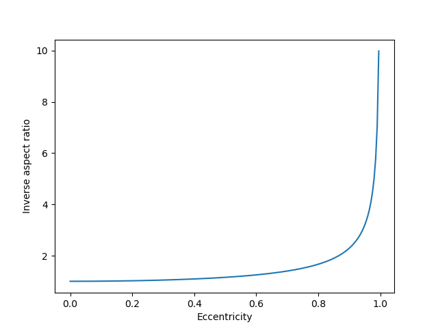
Mean anomaly, true anomaly, and eccentric anomaly are three ways of describing where an object is in its orbit. All would be the same if planets moved in circular orbits. And since planets nearly do move in circular orbits [1], at least in our solar system, these three anomalies will be similar. We will demonstrate this with plots.

Mean anomaly

Suppose a planet orbiting a star has period T, i.e. it takes time T for the planet to complete one orbit. Let t0 be the time when the planet was closest to the star, i.e. the time since the planet passed through periapsis [2]. Let t be the current time. Then the mean anomaly M is simply

M = 2π(tt0) / T

if you’re working in radians. Change 2π to 360° if you’re working in degrees.

True anomaly

The true anomaly f is the angle with vertex at the star and sides running from the star to periapsis and from the star to the planet. (I don’t know why true anomaly is denoted f. I suppose t and T were taken.)

Eccentric anomaly

The eccentric anomaly E is sorta like the true anomaly, but with the vertex at the center of the elliptical orbit rather than at the star. I say sorta because that’s not quite right.

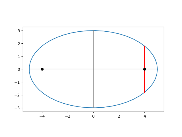
The eccentric anomaly is an angle with vertex at the center of the elliptical orbit. (The star is not at the center because elliptical orbits are eccentric, literally off-center.) One side does run along the major axis as with the true anomaly, but the other side doesn’t extend from the center to the planet but rather from the center to a projection of the planet’s orbit onto a circle.

Imagine an elliptical orbit in the plane, centered at the origin, with major axis along the x-axis. Now draw a circle around the ellipse with radius equal to the semi-major axis of the ellipse. So the circle touches the ellipse on the two ends, apsis and periapsis, but otherwise extends above and below the ellipse. Take a point P in the orbit and push it out vertically to a point P‘ on the circumscribed circle. That is, keep the x coordinate of P the same, but push the y coordinate up if it’s positive, or down if it’s negative, to get a point on the circle.

Equations

Kepler’s equation relates mean anomaly and eccentric anomaly:

M = Ee sin E

where M is the mean anomaly, E is the eccentric anomaly, and e is the eccentricity of the orbit. So when e is small, M is approximately equal to E.

True anomaly f is related to eccentric anomaly by

f = E + 2 arctan( β sin E / (1 − β cos E) )

where

β = e / (1 + √(1 − e²)).

I’ve written about Kepler’s equation a couple times. Here is a post about a simple way to solve Kepler’s equation for E given M, and here is a post about more efficient ways to solve Kepler’s equation.

Examples

Let’s make some plots comparing mean anomaly, eccentric anomaly, and true anomaly. Mean anomaly is proportional to time, so we’ll use it as our independent variable. Eccentric anomaly and true anomaly are roughly equal to mean anomaly, so we’ll plot the difference between these anomaly and mean anomaly.

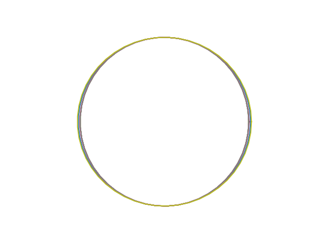
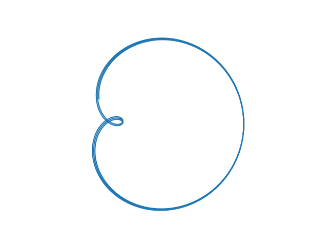
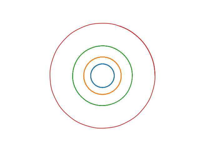
Here’s what we get for Earth, e = 0.01671.

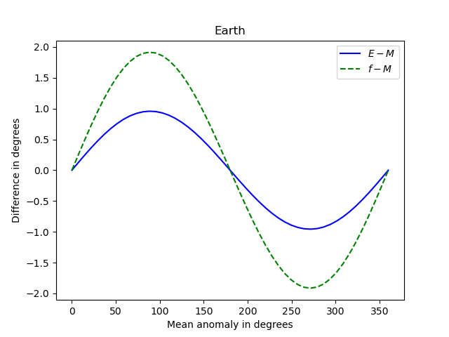
Note that the three anomalies never differ by more than 2 degrees.

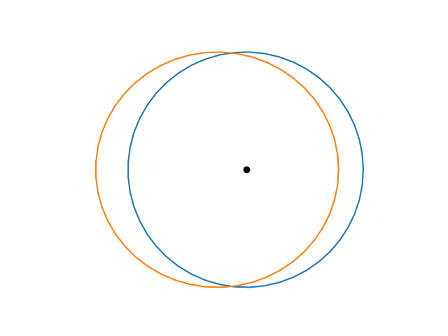
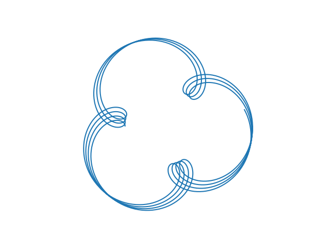
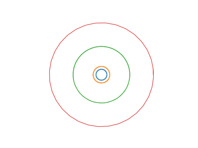
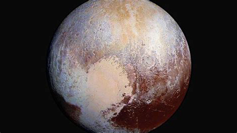
And here’s what we get for Pluto, e = 0.25.

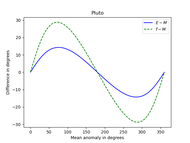
Now the differences between the anomalies is about 15 times greater. The shapes of the curves are roughly the same, but the curves for Earth are more symmetric about their peak and their trough than the corresponding curves for Pluto.

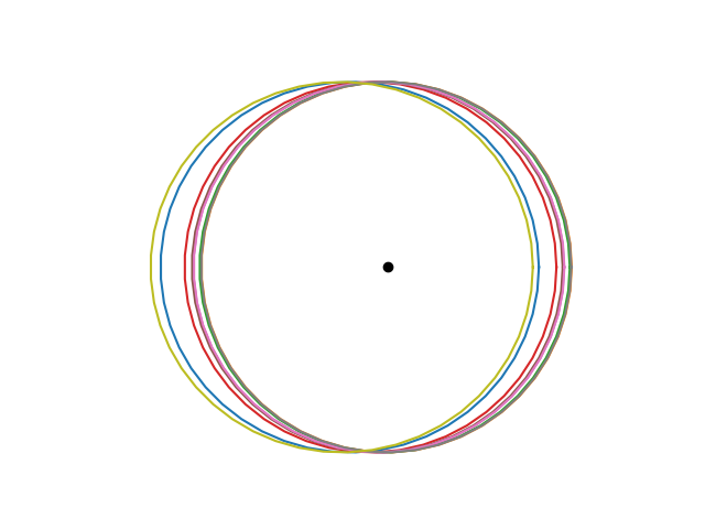
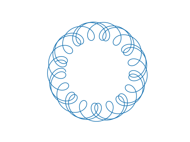
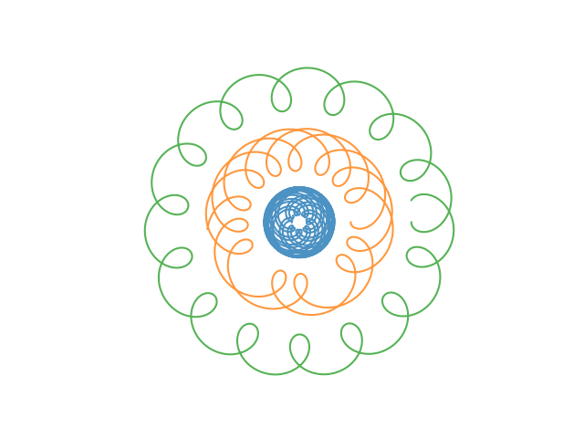
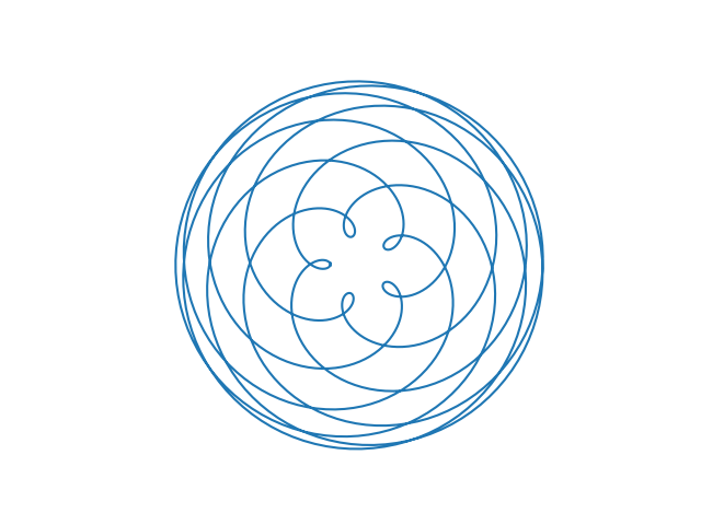
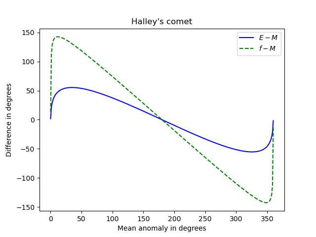
And here’s an extreme example: Halley’s comet. Its orbit has very high eccentricity, e = 0.967.

Newton’s method

I used Newton’s method to solve Kepler’s equation when making the plots above, using the mean anomaly as the initial guess when solving for the eccentric anomaly. I thought I might run into problems with high eccentricity, but everything worked smoothly, even for Halley’s comet. I suppose the basin of attraction for Newton’s method applied to Kepler’s equation is large, at least large enough to include mean anomaly as a starting point.

I didn’t even supply the root-finding method with a derivative functon. I used scipy.optimize.newton with just the function and starting point as arguments, letting the routine construct its own approximate derivative.

Notes

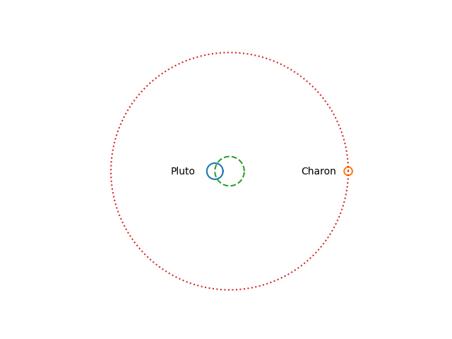
[1] The planets in our solar system move in very nearly circular orbits as explained here. The dwarf planet Pluto has a rather eccentric orbit (e = 0.25) and yet its orbit isn’t far from circular. However, the center of its orbit is far from the sun, as explained here.

[2] This point goes by many names in different contexts. The generic term for this point is called periapsis. For a satellite orbiting the earth it’s called perigee. For an object orbiting our sun it’s called perihelion. For an object orbiting our moon it’s called perilune. …

Cryptography, hydrodynamics, and celestial mechanics

V. I. Arnold

Last night I was reading a paper by the late Russian mathematician V. I. Arnold “Polymathematics: is mathematics a single science or a set of arts?” and posted a lightly edited extract of it on Twitter. It begins

All mathematics is divided into three parts: cryptography, hydrodynamics, and celestial mechanics.

Arnold is alluding to the opening line to Julius Caesar’s Gallic Wars [1] which suggests he’s being a little playful. The unedited version leaves no doubt that he’s being playful or cynical.

All mathematics is divided into three parts: cryptography (paid for by CIA, KGB and the like), hydrodynamics (supported by manufacturers of atomic submarines), and celestial mechanics (financed by military and other institutions dealing with missiles, such as NASA).

I edited out the parenthetical remarks, in part edit the sentence down to a tweet, but also because when you take out the humor/cynicism he makes a valid if hyperbolic point. He goes on to back this up.

Cryptography has generated number theory, algebraic geometry over finite fields, algebra, combinatorics and computers.

Hydrodynamics has procreated complex analysis, partial differential equations, Lie groups and algebra theory, cohomology theory and scientific computing.

Celestial mechanics is the origin of dynamical systems, linear algebra, topology, variational calculus and symplectic geometry.

Arnold adds a footnote to the comment about cryptography:

The creator of modern algebra, Viète, was the cryptographer of King Henry IV of France.

Of course not all mathematics was motivated by cryptography, hydrodynamics, and celestial mechanics, but an awful lot of it was. And his implicit argument that applied math gives birth to pure math is historically correct. Sometimes pure math gives rise to applied math, but much more often it’s the other way around.

His statements roughly match my own experience. Much of the algebra and number theory that I’ve learned has been motivated by cryptography. I dove into Knuth’s magnum opus, volume 2, because I wanted to implement the RSA algorithm in C++.

I got started in scientific computing in a computational fluid dynamics (CDF) lab. I didn’t work in the lab, but my roommate did, and I went there to use the computers. That’s where I would try my hand at numerical analysis and where I wrote simulation code for my dissertation. My dissertation in partial differential equations was related (very abstractly) to fluid flow in porous media.

I didn’t know anything about celestial mechanics until I sat in on Richard Arenstorf‘s class as a postdoc. So celestial mechanics was not my personal introduction to dynamical systems etc., but Arnold is correct that these fields came out of celestial mechanics.

Related posts

[1] “Gallia est omnis divisa in partes tres.” which translates “Gaul is a whole divided into three parts.”

How eccentricity matters

I wrote last week that the eccentricities of planet orbits in our solar system do not effect the shape of the orbit very much. Here’s a plot of all the orbits, shifted to have the same center and scaled to have the same minor axis.


However, the planet orbits do not have a common center. The eccentricity of an orbit doesn’t affect its shape as much as its position. Eccentric orbits are off-center. That’s literally what eccentric means.

Kepler’s laws say that each planet orbits in an ellipse with the sun at one focus of that ellipse. That means the more eccentric an orbit is, the further the center of the orbit is from the sun.

If a planetary orbit has semi-major axis a and the foci are a distance c from the center, then the eccentricity e equals c/a. If we scale all the planetary orbits so that they each have a semi-major axis equal to 1, then e = c, i.e. the eccentricity equals the distance from each focus to the center.

Imagine the sun as the center of our coordinate system and that each planet’s orbit is aligned so that its major axis is along the x axis. Each orbit has the sun, i.e. the origin, as a focus, and so the center of each orbit is at –e where e is the eccentricity of that orbit. Here’s the plot above redone to fix the sun rather than to fix the center. The black dot in the center is the sun.

Here is the same plot with only Venus and Pluto.

The orbit of Venus is essentially a circle centered at the sun. The orbit of Pluto is an ellipse with major axis about 3% longer than its minor axis. It’s hard to see that the shape of Pluto’s orbit is not a circle, but it’s easy to see that the orbit is off-center, i.e. eccentric.

This post explains why moderately large eccentricities do not have much impact on the aspect ratio of an ellipse.

The image below from this post shows an ellipse with eccentricity 0.8. The two foci are far from the center, and yet the the aspect ratio is 3 : 5. It’s obviously an ellipse, but the foci are further apart than you might imagine.


The view from a Galilean moon

The Galilean moons are the four largest moons of Jupiter, first observed by Galileo, contra Stigler’s law of eponymy.

This post shows what the Jovian system look like from the perspective of each of these moons, a sort of pre-Copernican perspective in a Jovian context.

The view from Io

Here’s what Europa would look like from Io. The orbital period for Europa is very nearly twice the orbital period of Io.

Here’s what Ganymede would look like from Io. The orbital period of Ganymede is very nearly 4 times that of Io.

Here’s what Callisto would look like from Io.

Here’s a combined view of the whole system, what Europa, Ganymede, Callisto, and Jupiter would look like from Io.

The view from Europa

The orbit of Io as seen from Europa is the same as the orbit of Europa as seen from Io.

Here’s what the orbit of Ganymede would look like from Europa. It’s similar to the view of Europa from Io because it is also a 2 : 1 resonance, i.e. the orbital period of Ganymede is approximately twice that of Europa.

Here’s what the orbit of Callisto would look like from Europa.

Here’s a combined view of the whole system, what Io, Ganymede, Callisto, and Jupiter would look like from Io.

The view from Ganymede

The view of Io from Ganymede is the same as the view of Ganymede from Io above. Similarly for Europa and Ganymede.

Here’s what the orbit of Callisto would look like from Ganymede. The two moons are in a 7 : 3 resonance.

Here’s a combined view of the whole system from Ganymede.

View of Callisto

The views of each of the moons from Callisto are presented above by symmetry. Here’s what the whole Jovian system would look like from Callisto.

View from Jupiter

Finally, here’s what the orbits of each of the moons looks like from Jupiter.

Related posts

What if Copernicus had been a Martian?

The genius of Copernicus was to realize that this plot

view of Mars, Jupiter, and Saturn from Earth

becomes this plot

View of Earth, Mars, Jupiter, and Saturn from the sun

under a clever change of coordinates.

The first plot is the apparent motion of Mars, Jupiter, and Saturn as viewed from Earth over the course of 30 years. Of course Copernicus knew of Mercury and Venus as well, but I’ve omitted them to make the plot simpler. The second plot is the view of Earth, Mars, Jupiter, and Saturn from the sun.

If Copernicus had lived on Mars, what view of the solar system would he have started with? Here’s what 30 (Earth) years of the apparent motion of Earth, Jupiter, and Saturn would look like from Mars.

View of Earth, Jupiter, and Saturn from Mars

These plots were produced by modifying the Python script given in the previous post.

How the orbit of one planet appears from another

This post shows how the orbits some planets appear from other planets. I’ve give a few of my favorite examples and include a Python program you could use to create your own plots.

We will assume the planets move in circles around the sun. They don’t exactly—they don’t exactly move in ellipses either—but their orbits are much closer to circles than most people realize. More on that here.

Venus / Earth

The ratio of Earth’s orbital period to that of Venus is almost exactly 13 to 8, so the view of Venus from Earth is nearly periodic with period 8 (Earth) years.

Venus from Earth

This is also the view of Earth from Venus. As the code below shows, the view of X from Y is the same as the view of Y from X.

Jupiter / Saturn

The ratio of Saturn’s orbital period to that of Jupiter is nearly 5 to 2. If this ratio were exactly, the figure below would repeat itself every two Saturnine years. But the following plot is over 4 Saturnine years, showing that years 3 and 4 don’t exactly retrace the path of years 1 and 2.

Jupiter from Saturn

Uranus / Earth

Here’s what the orbit of Uranus looks like from Earth.

Uranus from Earth

We see a big circle of tight little circles because the ratio of the distances from the sun is large.

Mercury / Venus

Here’s what Mercury looks like from Venus.

Mercury from Venus

Jovian moons

The same math that describes planets around the sun describes moons orbiting a planet. Here is what the orbit of Ganymede looks like from Callisto, and vice versa, as they orbit Jupiter. Ganymede completes 7 orbits in the time it takes Callisto to complete 3 orbits.

Ganymede and Callisto

Python code

Here’s the code that produced the plots.

    import matplotlib.pyplot as plt
    from numpy import linspace, sin, cos, pi
    
    period = {
        'mercury' : 87.96926,
        'venus'   : 224.7008,
        'earth'   : 365.25636,
        'mars'    : 686.97959,
        'ceres'   : 1680.22107,
        'jupiter' : 4332.8201,
        'saturn'  : 10755.699,
        'uranus'  : 20687.153,
        'neptune' : 60190.03
    }
    
    dist = lambda T : T**(2/3) # Kepler
    
    def plot_orbit(planet1, planet2, periods=10):
        T1 = period[planet1]
        T2 = period[planet2]
        d1 = dist(T1)
        d2 = dist(T2)

        theta = linspace(0, 2*pi*periods, 1000)
        x = d1*cos(T2*theta/T1) - d2*cos(theta)
        y = d1*sin(T2*theta/T1) - d2*sin(theta)

        plt.gca().set_aspect("equal")
        plt.axis('off')
        plt.plot(x, y)
        plt.show()
    
    plot_orbit("venus", "earth", 8)
    plot_orbit("jupiter", "saturn", 4)
    plot_orbit("uranus", "earth", 57)
    plot_orbit("mercury", "venus", 9)

Eccentricity, Flattening, and Aspect Ratio

There are at least three common ways to describe the shape of an ellipse: eccentricity e, flattening f, and aspect ratio r. Each is a number between 0 and 1. (Flattening is also called ellipticity, which is a descriptive name, but unfortunately it sounds a lot like eccentricity.)

Although converting between these three descriptions is simple, it’s also a little counterintuitive. In particular, moderately large values of eccentricity correspond to small values of flattening. The previous post looked at how similar the orbits of all the planets are when you plot them all on the same scale. This is true even though the eccentricity of Venus is essentially 0 and the eccentricity of Pluto is 0.25.

Let a be the semi-major axis of the ellipse, the distance from the center to the furthest point of the ellipse.

Let b be the semi-minor axis of the ellipse, the distance from the center to the closest point on the ellipse.

Then the aspect ratio, flattening, and eccentricity are defined as follows:

\begin{align*} r &= \frac{b}{a} \\ f &= \frac{a-b}{a} \\ e &= \sqrt{1 - \frac{b^2}{a^2}} \\ \end{align*}

If we plot the orbits of all the planets, scaled so that b = 1 for all planets, then the distance to the furthest point in the orbit is 1/r. Here’s a graph of how 1/r varies as a function of e.

Notice that 1/r hardly changes as e varies between, say, 0 and 0.4. So saying that Pluto has a “highly elliptical” orbit with e = 0.25 does not mean that the shape of its orbit is far from a circle. Here’s a plot of all the planet orbits in our solar system, or all the planet orbits plus the orbit of Pluto if you’d like to be pedantic.

Converting between eccentricity, flattening, and aspect ratio

I made the comment on Twitter that the orbit of the earth around the sun is closer to being an exact circle than the lines of constant longitude are. This means that the fact that the earth’s equatorial bulge is more geometrically significant than the elliptical nature of our orbit.

If you want to confirm this statement, you’ll need to know the shape of earth’s orbit and the shape of a meridian. But you’re most likely to find the former described in terms of eccentricity and the latter in terms of flattening. This is an example of why you might want to convert between different ways of describing the shape of an ellipse. Here are the conversion formulas.

\begin{align*} e &= \sqrt{2f - f^2} \\ e &= \sqrt{1-r^2} \\ f &= 1-\sqrt{1-e^2} \\ f &= 1-r \\ r &= \sqrt{1-e^2} \\ r &= 1-f \\ \end{align*}

According to Wikipedia, the eccentricity of earth’s orbit is 0.01671 and the flattening is 1/298.3. To put these on a common scale, meridians have eccentricity: 0.08181, about five times the eccentricity of earth’s orbit.

Similarly, the earth’s orbit has flattening 0.00013962 or about 24 times the flattening of the meridians.

So you could say earth’s orbit is 4 times or 24 times closer to being a circle than earth’s meridians are. The two ratios are very different because the conversion between eccentricity and flattening is highly nonlinear.

Related posts

Planetary orbits are very nearly circular

If a science book shows you obviously elliptical orbits of planets, it is literally stretching the truth.

I was taught that our benighted ancestors insisted that planetary orbits are circles for philosophical reasons. In fact, they insisted planetary orbits are circular because they very nearly are.

Here’s a plot of the orbits of all nine planets in our solar system, or all eight planets and the dwarf planet Pluto if you prefer, scaled so that they all have the same semi-minor axis.

See how far the “highly elliptical” orbit of Pluto extends past the perfect circle in the inside? Me neither.

Here is how Kepler discovered that planets have elliptical orbits [1].

From 1601 to 1608, he [Kepler] tried fitting various geometrical curves to Tycho’s data on the positions of Mars. Finally, after struggling for almost a year to remove a discrepancy of of 8 minutes of arc (which a less honest man might have chosen to ignore!) Kepler hit upon the ellipse as a possible solution.

It was only by obsessing over a discrepancy of 0.037% of a circle that Kepler was able to discover that Mars has an elliptical orbit.

The next post explains why eccentricity numbers are misleading. The orbit of Pluto, for example, is “highly eccentric” with eccentricity 0.25, but this does not result in an orbit far from circular.

[1] Roger Bate et al. Fundamentals of Astrodynamics. Dover. 1971

The Pluto-Charon orbit

The Moon doesn’t orbit the center of the Earth; it orbits the center of mass of the Earth-Moon system, which is inside the Earth. The distinction matters for designing satellite orbits, but it cannot be seen on a plot to scale. We’ll quantify this below.

Pluto’s moon Charon, however, is so large relative to Pluto and so close, that the center of mass of the Pluto-Charon system is outside of Pluto, and you can easily see this in a plot.

Plot of Pluto and Charon orbiting their barycenter

Imagine Pluto and Charon sitting on each end of a balanced seesaw. Pluto is a distance x1 to the left of the fulcrum, and Charon is a distance x2 to the right of the fulcrum. Let m1 be the mass of Pluto and m2 be the mass of Charon. Then

m1 x1 = m2 x2

and

x1 = m2 (x1 + x2) / (m1 + m2).

Now let’s put in some numbers.

m1 = 1.309 × 10²² kg
m2 = 1.62 × 1021 kg
x1 + x2 = 19,640 km

From this we find

x1 = (1.62 × 19640 / 14.71) km = 2163 km

and so the distance from the center of Pluto to the center of mass of the Pluto-Charon system is 2163 km. But the radius of Pluto is only 1190 km. So the center of mass of the Pluto-Charon system is about as far above the surface of Pluto as the center of Pluto is below the surface.

Comparison with the Earth-Moon system

It matters that the moon doesn’t exactly orbit the center of the Earth, but the difference between the center of the Earth and the center of mass of the Earth-Moon system is less dramatic. Let’s put in the numbers for the Earth and Moon.

m1 = 5.97 × 1024 kg
m2 = 7.346 × 1022 kg
x1 + x2 = 392,600 km

From this we find

x1 = (7.346 × 392,600 / 604) km = 4,775 km

The radius of Earth is 6,371 km, and so the center of mass of the Earth-Moon system is inside the Earth.

I made a plot analogous to the one above but for the Earth-Moon system. You could barely see the moon because it is so small relative to the size of its orbit. And you cannot see the difference between the center of the Earth and the barycenter of the Earth and Moon.

Tidal locking

Not only is Charon tidally locked with Pluto, as our moon is with Earth, but Pluto is tidally locked with Charon as well.

On Earth we only ever see one side of the moon. We never see the “dark side,” which is more accurately the “far side.” But someone standing on the moon would see Earth rotate.

Someone standing on Pluto would only ever see one side of Charon, and someone standing on Charon would only ever see one side of Pluto. Sputnik Planitia, the big heart-shaped feature on Pluto, is on the opposite side of Charon, so you could say Pluto is hiding its heart from its companion.

Image of Pluto featuring heart-shaped region

More orbital mechanics posts

Shape of moon orbit around sun

The earth’s orbit around the sun is nearly a circle, and the moon’s orbit around the earth is nearly a circle, but what is the shape of the moon’s orbit around the sun?

You might expect it to be bumpy, bending inward when the moon is between the earth and the sun and bending output when the moon is on the opposite side of the earth from the sun. But in fact the shape of the moon’s orbit around the sun is convex as proved in [1] and illustrated below.

If the moon orbited the earth much faster, say 10 times faster, at the same altitude, then we see that the orbit is indeed bumpy.

However, the nothing could orbit the earth 10x faster than the moon at the same distance as the moon. Orbital period determines altitude and vice versa.

A more realistic example would be a satellite in MEO (Medium Earth Orbit) like a GPS satellite. Such a satellite orbits the earth roughly twice a day. The path of a MEO satellite around the sun is not convex.

The plot above shows about one day of an MEO satellite’s orbit around the sun. Note that the vertical and horizontal scales are not the same; it would be hard to see anything but a flat line if the scales were the same because the satellite is far closer to the earth than the sun.

Here are the equations from [1]. Choose units so that the distance to the moon or satellite is 1 and let d be the distance from the planet to the sun. Let p be the number of times the moon or satellite orbits the planet as the planet orbits the sun (the number of sidereal periods).

x(θ) = d cos(θ) + cos(pθ)
y(θ) = d sin(θ) + sin(pθ)

This assumes both the planet’s orbit around the sun and the satellite’s orbit around the planet are circular, which is a good approximation in our examples.

[1] Noah Samuel Brannen. The Sun, the Moon, and Convexity. The College Mathematics Journal, Vol. 32, No. 4 (Sep., 2001), pp. 268-272