The Galilean moons are the four largest moons of Jupiter, first observed by Galileo, contra Stigler’s law of eponymy.
This post shows what the Jovian system look like from the perspective of each of these moons, a sort of pre-Copernican perspective in a Jovian context.
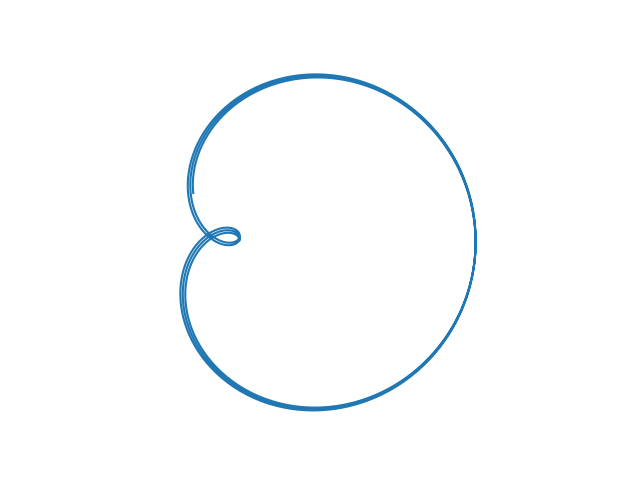
The view from Io
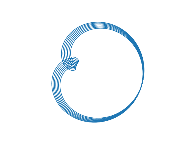
Here’s what Europa would look like from Io. The orbital period for Europa is very nearly twice the orbital period of Io.
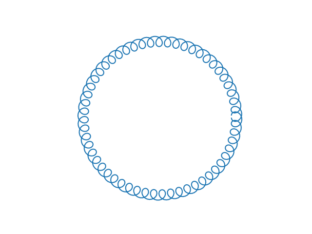
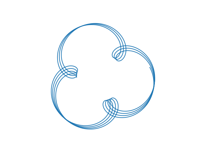
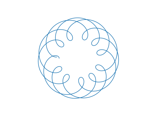
Here’s what Ganymede would look like from Io. The orbital period of Ganymede is very nearly 4 times that of Io.
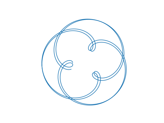
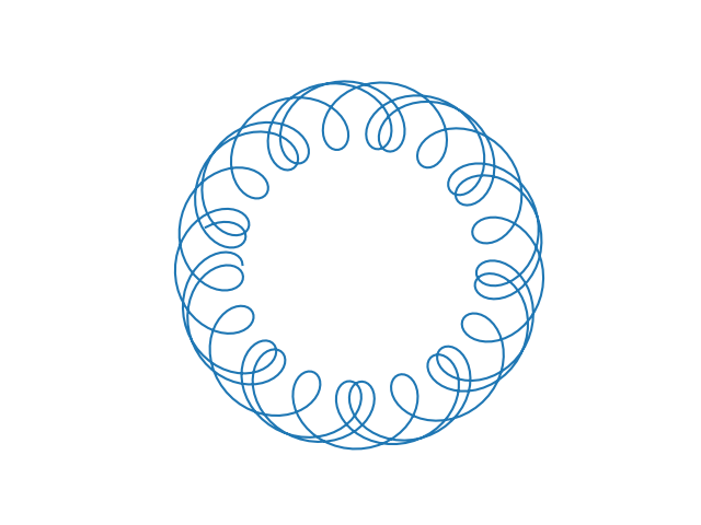
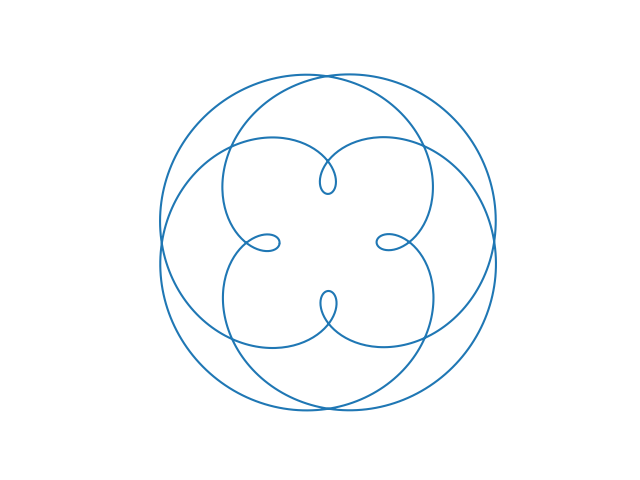
Here’s what Callisto would look like from Io.
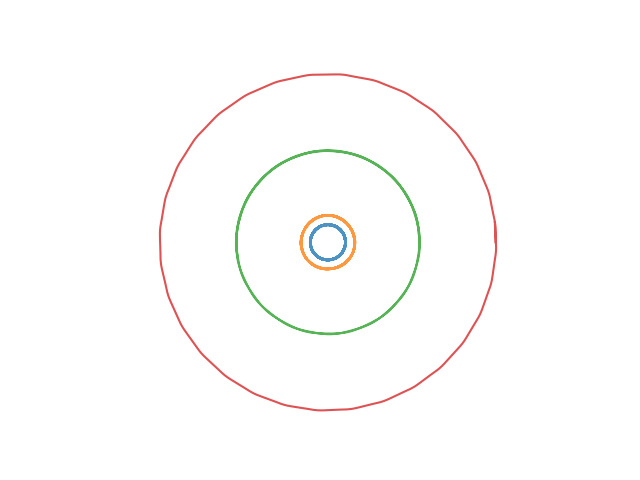
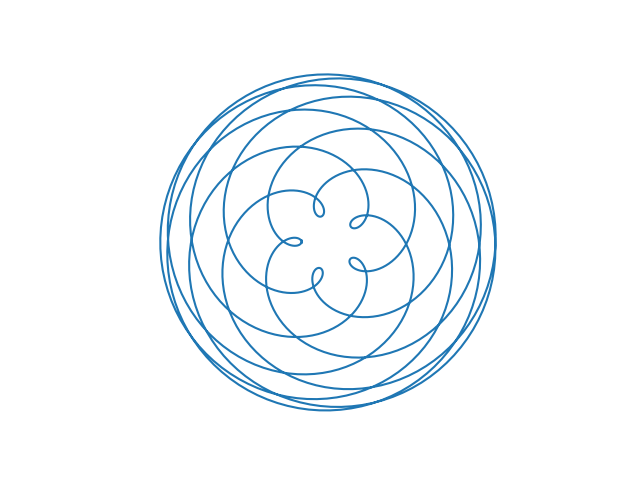
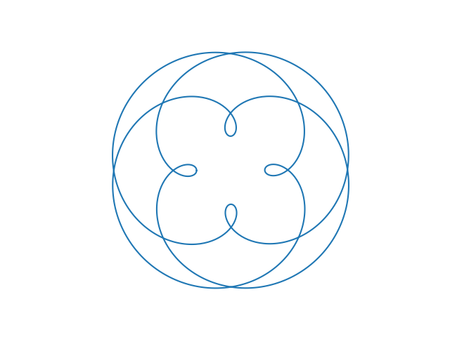
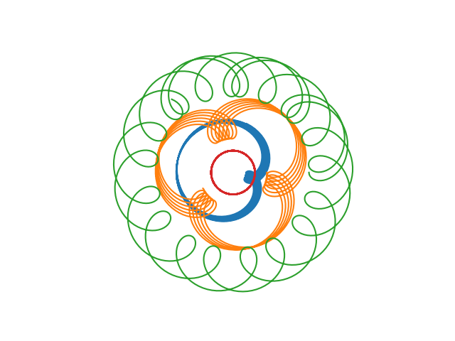
Here’s a combined view of the whole system, what Europa, Ganymede, Callisto, and Jupiter would look like from Io.
The view from Europa
The orbit of Io as seen from Europa is the same as the orbit of Europa as seen from Io.
Here’s what the orbit of Ganymede would look like from Europa. It’s similar to the view of Europa from Io because it is also a 2 : 1 resonance, i.e. the orbital period of Ganymede is approximately twice that of Europa.
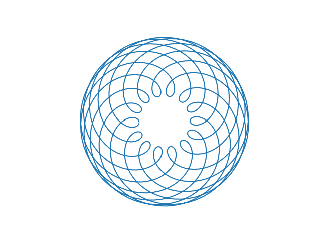
Here’s what the orbit of Callisto would look like from Europa.
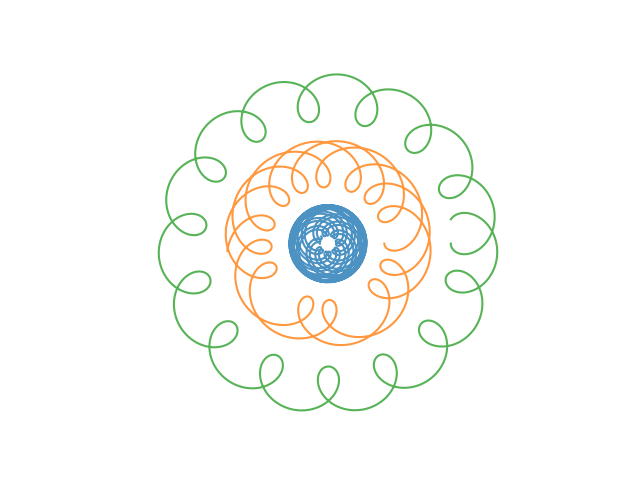
Here’s a combined view of the whole system, what Io, Ganymede, Callisto, and Jupiter would look like from Io.
The view from Ganymede
The view of Io from Ganymede is the same as the view of Ganymede from Io above. Similarly for Europa and Ganymede.
Here’s what the orbit of Callisto would look like from Ganymede. The two moons are in a 7 : 3 resonance.
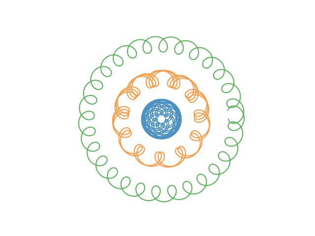
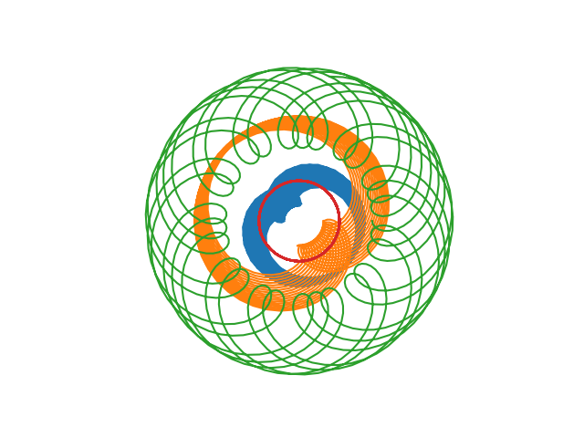
Here’s a combined view of the whole system from Ganymede.
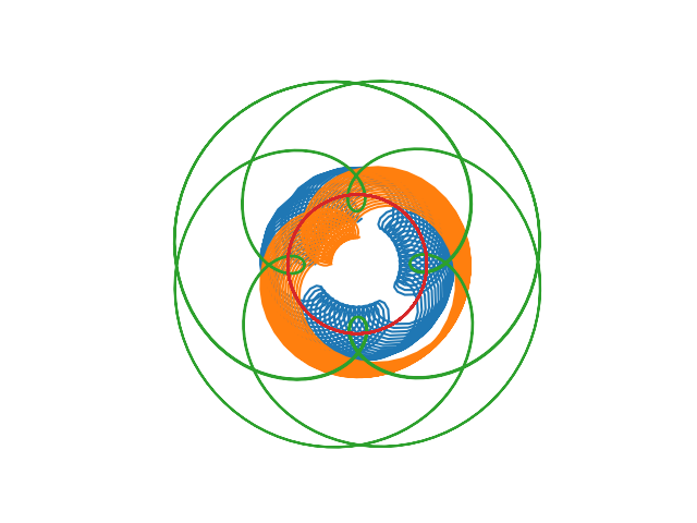
View of Callisto
The views of each of the moons from Callisto are presented above by symmetry. Here’s what the whole Jovian system would look like from Callisto.
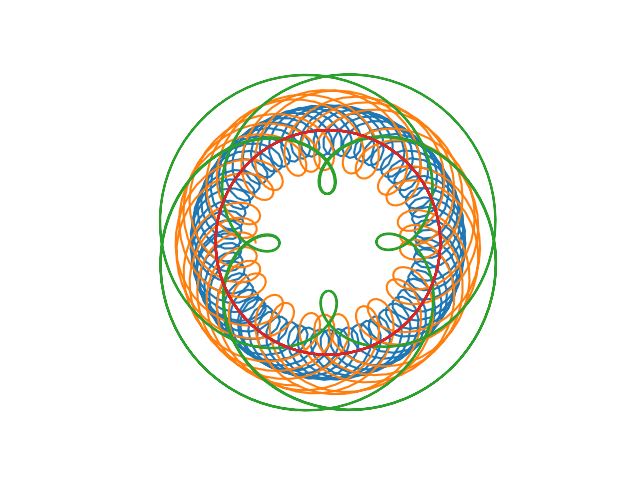
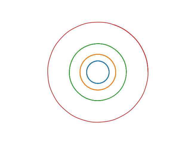
View from Jupiter
Finally, here’s what the orbits of each of the moons looks like from Jupiter.