A shell one-liner to search directories

Posted on 19 April 2020 by John

I started this post by wanting to look at the frequency of LaTeX commands, but then thought that some people mind find the code to find the frequencies more interesting than the frequencies themselves.

So I’m splitting this into two posts. This post will look at the shell one-liner to find command frequencies, and the next post will look at the actual frequencies.

I want to explore LaTeX files, so I’ll start by using find to find such files.

    find . -name "*.tex"

This searches for files ending in .tex, starting with the current directory (hence .) and searching recursively into subdirectories. The find command explores subdirectories by default; you have to tell it not to if that’s not what you want.

Next, I want to use grep to search the LaTeX files. If I pipe the output of find to grep it will search the file names, but I want it to search the file contents. The xargs command takes care of this, receiving the file names and passing them along as file names, i.e. not as text input.

    find . -name "*.tex" | xargs grep ...

LaTeX commands have the form of a backslash followed by letters, so the regular expression I’ll pass is \\[a-z]+. This says to look for a literal backslash followed by one or more letters.

I’ll give grep four option flags. I’ll use -i to ask it to use case-insensitive matching, because LaTeX commands can begin contain capital letters. I’ll use -E to tell it I want to use extended regular expressions [1].

I’m after just the commands, not the lines containing commands, and so I use the -o option to tell grep to return just the commands, one per line. But that’s not enough. It would be enough if we were only search one file, but since we’re searching multiple files, the default behavior is for grep to return the file name as well. The -h option tells it to only return the matches, no file names.

So now we’re up to this:

    find . -name "*.tex" | xargs grep -oihE '\\[a-z]+'

Next I want to count how many times each command occurs, and I need to sort the output first so that uniq will count correctly.

    find . -name "*.tex" | xargs grep -oihE '\\[a-z]+' | sort | uniq -c

And finally I want to sort the output by frequency, in descending order. The -n option tells sort to sort numerically, and -r says to sort in descending order than the default ascending order. This produces a lot of output, so I pipe everything to less to view it one screen at a time.

    find . -name "*.tex" | xargs grep -oihE '\\[a-z]+' | sort | uniq -c | sort -rn | less

That’s my one-liner. In the next post I’ll look at the results.

Expected length of longest common DNA substrings

Posted on 18 April 2020 by John

If we have two unrelated sequences of DNA, how long would we expect the longest common substring of the two sequences to be? Since DNA sequences come from a very small alphabet, just four letters, any two sequences of moderate length will have some common substring, but how long should we expect it to be?

Motivating problem

There is an ongoing controversy over whether the SARS-CoV-2 virus contains segments of the HIV virus. The virologist who won the Nobel Prize for discovering the HIV virus, Luc Montagnier, claims it does, and other experts claim it does not.

I’m not qualified to have an opinion on this dispute, and do not wish to discuss the dispute per se. But it brought to mind a problem I’d like to say something about.

This post will look at a simplified version of the problem posed by the controversy over the viruses that cause COVID-19 and AIDS. Namely, given two random DNA sequences, how long would you expect their longest common substring to be?

I’m not taking any biology into account here other than using an alphabet of four letters. And I’m only looking at exact substring matches, not allowing for any insertions or deletions.

Substrings and subsequences

There are two similar problems in computer science that could be confused: the longest common substring problem and the longest common subsequence problem. The former looks for uninterrupted matches and the latter allows for interruptions in matches in either input.

For example, “banana” is a subsequence of “bandana” but not a substring. The longest common substring of “banana” and “anastasia” is “ana” but the longest common subsequence is “anaa.” Note that the latter is not a substring of either word, but a subsequence of both.

Here we are concerned with substrings, not subsequences. Regarding the biological problem of comparing DNA sequences, it would seem that a substring is a strong form of similarity, but maybe too demanding since it allows no insertions. Also, the computer science idea of a subsequence might be too general for biology since it allows arbitrary insertions. A biologically meaningful comparison would be somewhere in between.

Simulation results

I will state theoretical results in the next section, but I’d like to begin with a simulation.

First, some code to generate a DNA sequence of length N.

    from numpy.random import choice

    def dna_sequence(N):
        return "".join(choice(list("ACGT"), N))

Next, we need a way to find the longest common substring. We’ll illustrate how SequenceMatcher works before using it in a simulation.

    from difflib import SequenceMatcher

    N = 12
    seq1 = dna_sequence(N)
    seq2 = dna_sequence(N)   
 
    # "None" tells it to not consider any characters junk
    s = SequenceMatcher(None, seq1, seq2)

    print(seq1)
    print(seq2)
    print(s.find_longest_match(0, N, 0, N))

This produced

    TTGGTATCACGG
    GATCACAACTAC
    Match(a=5, b=1, size=5)

meaning that the first match of maximum length, ATCAC in this case, starts in position 5 of the first string and position 1 of the second string (indexing from 0).

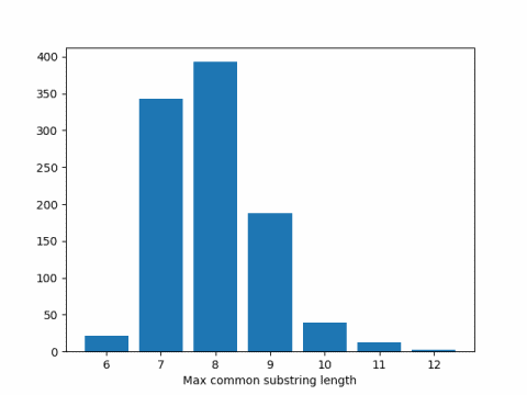
Now let’s run a simulation to estimate the expected length of the longest common substring in two sequences of DNA of length 300. We’ll do 1000 replications of the simulation to compute our average.

    def max_common_substr_len(a, b):
        # The None's turn off junk detection heuristic
        s = SequenceMatcher(None, a, b, None)
        m = s.find_longest_match(0, len(a), 0, len(b))
        return m.size

    seqlen = 300
    numreps = 1000
    avg = 0
    for _ in range(numreps):
        a = dna_sequence(seqlen)
        b = dna_sequence(seqlen)
        avg += max_common_substr_len(a, b)
    avg /= numreps
    print(avg)

When I ran this code I got 7.951 as the average. Here’s a histogram of the results.

Expected substring length

Arratia and Waterman [1] published a paper in 1985 looking at the longest common substring problem for DNA sequences, assuming each of the four letters in the DNA alphabet are uniformly and independently distributed.

They show that for strings of length N coming from an alphabet of size b, the expected length of the longest match is asymptotically

2 log_b(N).

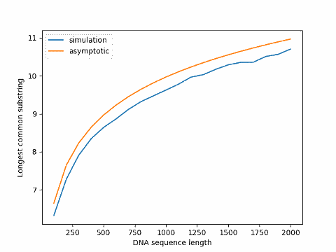
This says in our simulation above, we should expect results around 2 log₄(300) = 8.229.

There could be a couple reasons our simulation results were smaller than the theoretical results. First, it could be a simulation artifact, but that’s unlikely. I repeated the simulation several times and consistently got results below the theoretical expected value. I expect Arratia and Waterman’s result, although exact in the limit, is biased upward for finite n.

Update: The graph below plots simulation results for varying sequence sizes compared to the asymptotic value, the former always below the latter.

Simulation vs asymptotic estimate

Arratia and Waterman first assume i.i.d. probabilities to derive the result above, then prove a similar theorem under the more general assumption that the sequences are Markov chains with possibly unequal transition probabilities. The fact that actual DNA sequences are not exactly uniformly distributed and not exactly independent doesn’t make much difference to their result.

Arratia and Waterman also show that allowing for a finite number of deletions, or a number of deletions that grows sufficiently slowly as a function of n, does not change their asymptotic result. Clearly allowing deletions makes a difference for finite n, but the difference goes away in the limit.

[1] Richard Arratia and Michael S. Waterman. An Erdős-Rényi Law with Shifts. Advances in Mathematics 55, 13-23 (1985).

Powers that don’t change the last digit

Posted on 14 April 2020 by John

If you raise any number to the fifth power, the last digit doesn’t change.

Here’s a little Python code to verify this claim.

    >>> [n**5 for n in range(10)]
    [0, 1, 32, 243, 1024, 3125, 7776, 16807, 32768, 59049]

In case you’re not familiar with Python, or familiar with Python but not familiar with list comprehensions, the code is very similar to set builder notation in math:

{n⁵ | n = 0, 1, 2, … 9}

To emphasize the last digits, we could take the remainder by 10:

    >>> [n**5 % 10 for n in range(10)]
    [0, 1, 2, 3, 4, 5, 6, 7, 8, 9]

The reason this works is related to Fermat’s little theorem.

We could generalize this to the last digits in other bases. For example, in base 21, raising numbers to the 13th power doesn’t change the last digit. You could verify this by running

    [x**13 % 21 for x in range(21)]

Why do we take 5th powers in base 10 and 13th powers in base 21? Because φ(10) + 1 = 5 and φ(21) + 1 = 13 where φ(m) is Euler’s “totient” function applied to the base. The function φ(m) is defined as the number of positive integers less than m that are relatively prime to m.

If we’re in base 30, φ(30) = 8, and so we’d expect 9th powers to leave the last digit unchanged. And we can evaluate

    [n**9 % 30 for n in range(30)]

to see that this is the case.

Now let’s try base 16. We have φ(16) = 8, so let’s raise everything to the 9th power.

    >>> [n**9 % 16 for n in range(16)]
    [0, 1, 0, 3, 0, 5, 0, 7, 0, 9, 0, 11, 0, 13, 0, 15]

That didn’t work out the way the other examples did. Why’s that? The bases 10, 21, and 30 are the product of distinct primes, but 16 is a prime power.

However, there’s something else interesting going on in base 16. Instead of taking the remainder by 16, i.e. looking at the last hexadecimal digit, let’s look at all the digits.

    >>> [hex(n**9) for n in range(16)]
    ['0x0', '0x1', '0x200', '0x4ce3', '0x40000', ..., '0x8f3671c8f']

In base 16, the last digit of n⁹ is not the same as the last digit of n. But the last non-zero digit is the same as the last digit of n.

An application of Kronecker products

Posted on 13 April 2020 by John

A while back I wrote about Kronecker products in the context of higher order Taylor series. Here’s how I described the Kronecker product in that post.

The Kronecker product of an m × n matrix A and a p × q matrix B is a mp × nq matrix K = A ⊗ B. You can think of K as a block partitioned matrix. The ij block of K is a_ijB. In other words, to form K, take each element of A and replace it with its product with the matrix B.

The post gives the example that if

$A = \left\[ \begin{array}{cc} 1 & 2 \\ 3 & 4 \\ 5 & 6 \\ 7 & 8 \end{array} \right]$

and

$B= \left\[ \begin{array}{ccc} 10 & 0 & 0 \\ 0 & 20 & 0 \\ 0 & 0 & 30 \end{array} \right]$

then

$A \otimes B= \left\[ \begin{array}{cccccc} 10 & 0 & 0 & 20 & 0 & 0 \\ 0 & 20 & 0 & 0 & 40 & 0 \\ 0 & 0 & 30 & 0 & 0 & 60 \\ 30 & 0 & 0 & 40 & 0 & 0 \\ 0 & 60 & 0 & 0 & 80 & 0 \\ 0 & 0 & 90 & 0 & 0 & 120 \\ 50 & 0 & 0 & 60 & 0 & 0 \\ 0 & 100 & 0 & 0 & 120 & 0 \\ 0 & 0 & 150 & 0 & 0 & 180 \\ 70 & 0 & 0 & 80 & 0 & 0 \\ 0 & 140 & 0 & 0 & 160 & 0 \\ 0 & 0 & 210 & 0 & 0 & 240 \\ \end{array} \right]$

That post used Kronecker products to express Taylor series for functions of several variables. This post will present another application of Kronecker products.

Hadamard matrices

Hadamard matrices come up frequently in coding theory. For example, the existence of certain codes depends on the existence of Hadamard matrices of a certain size. These matrices also come up in the design of experiments. See Nick Higham’s recent article for applications to numerical linear algebra.

It’s important in application to know when Hadamard matrices exist and to be able to construct them. And the simplest way to construct Hadamard matrices is by taking Kronecker products of smaller Hadamard matrices.

A Hadamard matrix is an orthogonal matrix whose entries are all either +1 or −1. For example, the following is a 2 by 2 Hadamard matrix:

    +1  +1
    +1  -1

Now there’s a theorem due to James Sylvester (1814–1897) that says the Kronecker product of two Hadamard matrices is another Hadamard matrix. So if we can find Hadamard matrices of order p and order q, we can take their Kronecker product to form a Hadamard matrix of order pq. In particular, we can take the Kronecker product of the matrix above with itself n times to form a Hadamard matrix of order 2ⁿ.

So, for example, taking the product once we get a matrix of order 4.

    +1  +1  +1  +1
    +1  -1  +1  -1
    +1  +1  -1  -1
    +1  -1  -1  +1

And taking the product once again we get a Hadamard matrix of order 8.

    +1  +1  +1  +1  +1  +1  +1  +1 
    +1  -1  +1  -1  +1  -1  +1  -1 
    +1  +1  -1  -1  +1  +1  -1  -1 
    +1  -1  -1  +1  +1  -1  -1  +1
    +1  +1  +1  +1  -1  -1  -1  -1 
    +1  -1  +1  -1  -1  +1  -1  +1 
    +1  +1  -1  -1  -1  -1  +1  +1 
    +1  -1  -1  +1  -1  +1  +1  -1

It’s not known for which n there exists a Hadamard matrix of order n, but the construction above shows that there exist Hadamard matrix of every order that’s a power of 2. If n > 2 then a necessary condition for the existence of a Hadamard matrix is that n is a multiple of 4. It is conjectured that this condition is also sufficient. At the time of writing, the smallest multiple of 4 for which no one has found a Hadamard matrix is 668.

Note that, for example, there are Hadamard matrices of order 20, but you cannot find one by multiplying Hadamard matrices of order 4 and 5, because there are no Hadamard matrices of order 5. So if you wanted to create a list of Hadamard matrices of various orders, Sylvester’s theorem would let you quickly fill in some entries, but then things would get much harder.

A wrinkle in Clojure

Posted on 11 April 2020 by John

Bob Martin recently posted a nice pair of articles, A Little Clojure and A Little More Clojure. In the first article he talks about how spare and elegant Clojure is.

In the second article he shows how to write a program to list primes using map and filter rather than if and while. He approaches the example leisurely, showing how to arrive at the solution in small steps understandable to someone new to Clojure.

The second article passes over a small wrinkle in Clojure that I’d like to say a little about. Near the top of the post we read

The filter function also takes a function and a list. (filter odd? [1 2 3 4 5]) evaluates to (1 3 5). From that I think you can tell what both the filter and the odd? functions do.

Makes sense: given a bunch of numbers, we pick out the ones that are odd. But look a little closer. We start with [1 2 3 4 5] in square brackets and end with (1 3 5) in parentheses. What’s up with that? The article doesn’t say, and rightfully so: it would derail the presentation to explain this subtlety. But it’s something that everyone new to Clojure will run into fairly quickly.

As long as we’re vague about what “a bunch of numbers” means, everything looks fine. But when we get more specific, we see that filter takes a vector of numbers and returns a list of numbers [1]. Or rather it can take a vector, as it does above; it could also take a list. There are reasons for this, explained here, but it’s puzzling if you’re new to the language.

There are a couple ways to make the filter example do what you’d expect, to either have it take a vector and return a vector, or to have it take a list and return a list. Both would have interrupted the flow of an introductory article. To take a vector and return a vector you could run

    (filterv odd? [1 2 3 4 5])

This returns the vector [1 3 5].

Notice we use the function filterv rather than filter. If the article had included this code, readers would ask “Why does filter have a ‘v’ on the end? Why isn’t it just called ‘filter’?”

To take a list and return a list you could run

    (filter odd? '(1 2 3 4 5))

This returns the list (1 3 5).

But if the article had written this, readers would ask “What is the little mark in front of (1 2 3 4 5)? Is that a typo? Why didn’t you just send it the list?” The little mark is a quote and not a typo. It tells Clojure that you are passing in a list and not making a function call.

One of the core principles of Lisp is that code and data use the same structure. Everything is a list, hence the name: LISP stands for LISt Processing. Clojure departs slightly from this by distinguishing vectors and lists, primarily for efficiency. But like all Lisps, function calls are lists, where the first element of the list is the name of the function and the remaining elements are arguments [2]. Without the quote mark in the example above, the Clojure compiler would look in vain for a function called 1 and throw an exception:

CompilerException java.lang.RuntimeException: Unable to resolve symbol: quote in this context, compiling: …

Since vectors are unambiguously containers, never used to indicate function calls, there’s no need for vectors to be quoted, which simplifies the exposition in an introductory article.

Exponential growth vs logistic growth

Posted on 9 April 2020 by John

This seems like a good time to discuss the difference between exponential growth and logistic growth as the covid19 pandemic is starting to look more like a logistic model and less like an exponential model, at least in many parts of the world [1]. This post is an expansion of a Twitter thread I wrote on AnalysisFact.

***

Nothing in the world grows exponentially forever.

The beginning of exponential growth is easier to understand that its end.

From the beginning there are factors that keep growth from being purely exponential, but they are negligible at first. They can be ignored for a while, but not forever.

A logistic model takes one limiting factor into account, but things could be much more complicated than that.

Even though logistic models are often more realistic than exponential models, I wouldn’t want someone to read this and say “Oh, I see. Epidemics (for example) aren’t exponential, they’re logistic.” A logistic model is still a simple idealization, more realistic than an exponential model, but still simplistic.

A system with exponential growth satisfies

That is, the rate of growth y‘ at any given time is proportional to the state y. If you have money invested at a fixed rate of interest, for example, the amount of interest you earn is proportional to how much you’ve invested.

A system with logistic growth satisfies

That is, the rate of growth is the proportional to the product of two things: the current state y and the complement of the current state 1 – y. For example, a simple epidemic model says the rate of spread is proportional to the product of the proportion of infected people and the proportion of uninfected people. The rate of infection slows down as there are fewer people who have not been exposed.

(Let me say one more time that this is a simplistic model. Please don’t read this then publish your own amateur analysis of a pandemic [2].)

Logistic growth applies to many things, not just epidemics. The spread of rumors, for example, is approximately logistic. The rate of spread depends on both the number of people spreading the rumor and the number of people who haven’t heard. Once most people have heard, the rate slows way down because people are sharing the rumor with others who have already heard.

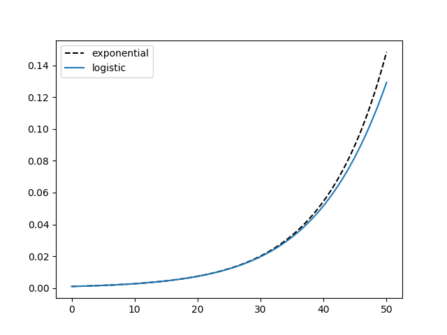
In the logistic differential equation above, when y is near 0, 1 − y is approximately 1 and so that term has little effect. That’s why logistic models look like exponential models at first. Here are plots of exponential and logistic models with y(0) = 0.001, k = 0.1, and time running from 0 to 50.

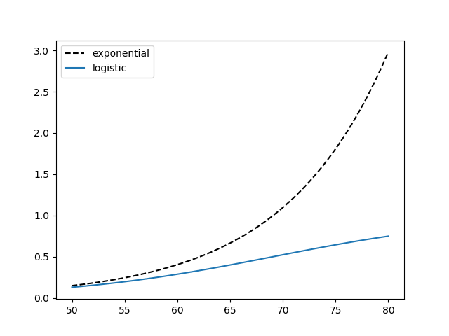
But the larger y gets, the more the 1 − y term matters more. Eventually it dominates. Here are the same functions for time running from 50 to 80.

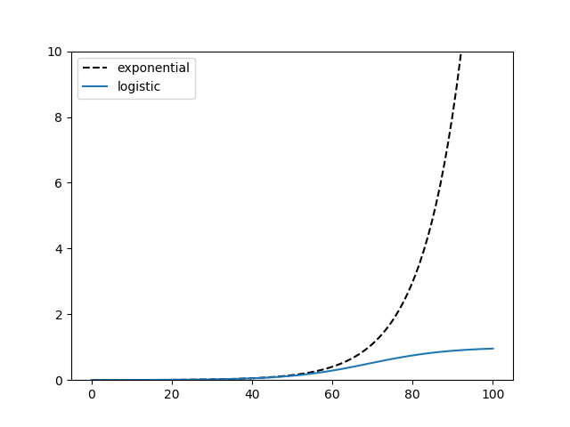
The logistic curve has a S shape and will flatten out, asymptotically approaching 1. Here’s a comparison of the two plots with time running from 0 to 100.

Sine series for a sine

Posted on 7 April 2020 by John

The Fourier series of an odd function only has sine terms—all the cosine coefficients are zero—and so the Fourier series is a sine series.

What is the sine series for a sine function? If the frequency is an integer, then the sine series is just the function itself. For example, the sine series for sin(5x) is just sin(5x). But what if the frequency is not an integer?

For an odd function f on [−π, π] we have

$f(x) = \sum_{n=0}^\infty c_n \sin(n x)$

where the coefficients are given by

$c_n = \frac{1}{\pi} \int_{-\pi}^\pi f(x) \sin(nx)\, dx$

So if λ is not an integer, the sine series coefficients for sin(λx) are given by

$c_n = 2\sin(\lambda \pi) (-1)^n \,\frac{ n}{\pi(\lambda^2 - n^2)}$

The series converges slowly since the coefficients are O(1/n).

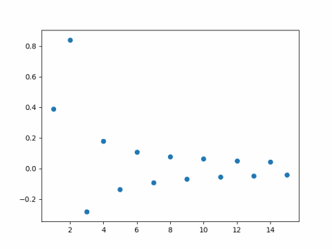
For example, here are the first 15 coefficients for the sine series for sin(1.6x).

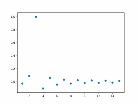
And here is the corresponding plot for sin(2.9x).

As you might expect, the coefficient of sin(3x) is nearly 1, because 2.9 is nearly 3. What you might not expect is that the remaining coefficients are fairly large.

Update: After writing this post I wrote another on the rate of convergence for Fourier series. In general, the smoother the function, the faster the Fourier series converges and vice versa, with some fine print.

The sine function above is perfectly smooth, but it’s Fourier series converges slowly. How can that be? The Fourier series is defined for periodic functions. If k is not an integer and we force sin(kx) to be a function with period 2π, it is not continuous. When we extend sin(kx) to make it periodic, there’s a jump discontinuity at the ends of each period.

Look back at

$f(x) = \sum_{n=0}^\infty c_n \sin(n x)$

This equation can’t hold everywhere. If k is not an integer and f(x) = sin(kx), then the right size is zero at π but the left is not. In fact we’ll see Gibbs phenomenon at π because of the discontinuity there.

Two meanings of QR code

Posted on 7 April 2020 by John

“QR code” can mean a couple different things. There is a connection between these two, though that’s not at all obvious.

What almost everyone thinks of as a QR code is a quick response code, a grid of black and white squares that encode some data. For example, the QR code below contains my contact info.

There’s also something in algebraic coding theory called a QR code, a quadratic residue code. These are error-correcting codes that are related to whether numbers are squares or not modulo a prime.

The connection between quick response codes and quadratic residue codes is that both involve error-correcting codes. However, quick response codes use Reed-Solomon codes for error correction, not quadratic residue codes. Reed-Solomon codes are robust to long sequences of error, which is important for quick response codes since, for example, a row of the image might be cut off. It would be cute if QR (quick response) codes used QR (quadratic residue) codes, but alas they don’t.

Center of mass and vectorization

Posted on 5 April 2020 by John

Para Parasolian left a comment on my post about computing the area of a polygon, suggesting that I “say something similar about computing the centroid of a polygon using a similar formula.” This post will do that, and at the same time discuss vectorization.

Notation

We start by listing the vertices starting anywhere and moving counterclockwise around the polygon:

$(x_1, y_1), (x_2, y_2), \cdots, (x_n, y_n)$

It will simplify notation below if we duplicate the last point:

The formula the centroid depends on the formula for the area, where the area of the polygon is

$A = \frac{1}{2} \sum_{i=0}^{n-1} (x_i y_{i+1} - x_{i+1}y_i)$

Hadamard product and dot product

We can express the area formula more compactly using vector notation. This will simplify the centroid formulas as well. To do so we need to define two ways of multiplying vectors: the Hadamard product and the dot product.

The Hadamard product of two vectors is just their componentwise product. This is a common operation in R or Python, but less common in formal mathematics. The dot product is the sum of the components of the Hadamard product.

If x and y are vectors, the notation xy with no further explanation probably means the dot product of x or y if you’re reading a math or physics book. In R or Python, x*y is the Hadamard product of the vectors.

Here we will use a circle ∘ for Hadamard product and a dot · for inner product.

Now let x with no subscript be the vector

$x = (x_0, x_1, x_2, \cdots, x_{n-1})$

and let x‘ be the same vector but shifted

$x' = (x_1, x_2, x_3, \cdots, x_n)$

We define y and y‘ analogously. Then the area is

$A = (x\cdot y' - x' \cdot y) / 2$

Centroid formula

The formula for the centroid in summation form is

$\begin{align*} C_x &= \frac{1}{6A} \sum_{i=0}^{n-1} (x_i + x_{i+1})(x_i y_{i+1} - x_{i+1}y_i) \\ C_y &= \frac{1}{6A} \sum_{i=0}^{n-1} (y_i + y_{i+1})(x_i y_{i+1} - x_{i+1}y_i) \end{align*}$

where A is the area given above.

We can write this in vector form as

$\begin{align*} C_x &= \frac{1}{6A} (x + x') \cdot (x\circ y' - x' \circ y) \\ C_y &= \frac{1}{6A} (y + y') \cdot (x\circ y' - x' \circ y) \\ \end{align*}$

You could evaluate v = x∘ y‘ – x‘∘y first. Then A is half the dot product of v with a vector of all 1’s, and the centroid x and y coordinates are inner products of v with x + x‘ and y + y‘ respectively, divided by 6A.

Making an invertible function out of non-invertible parts

Posted on 4 April 2020 by John

How can you make an invertible function out of non-invertible parts? Why would you want to?

Encryption functions must be invertible. If the intended recipient can’t decrypt the message then the encryption method is useless.

Of course you want an encryption function to be really hard to invert without the key. It’s hard to think all at once of a function that’s really hard to invert. It’s easier to think of small components that are kinda hard to invert. Ideally you can iterate steps that are kinda hard to invert and create a composite that’s really hard to invert.

So how do we come up with components that are kinda hard to invert? One way is to make small components that are non-linear, and that are in fact impossible to invert [1]. But how can you use functions that are impossible to invert to create functions that are possible to invert? It doesn’t seem like this could be done, but it can. Feistel networks, named after cryptographer Horst Feistel, provide a framework for doing just that.

Many block encryption schemes are based on a Feistel network or a modified Feistel network: DES, Lucifer, GOST, Blowfish, LOKI, etc.

The basic idea of Feistel networks is so simple that it may go by too fast the first time you see it.

You take a block of an even number of bits and split it into two sub-blocks, the left half L and the right half R. The nth round of a Feistel cipher creates new left and right blocks from the left and right blocks of the previous round by

$\begin{align*} L_n =& R_{n-1} \\ R_n =& L_{n-1} \oplus f(R_{n-1}, K_n) \end{align*}$

Here ⊕ is bitwise XOR (exclusive or) and f(R_n−1, K_n) is any function of the previous right sub-block and the key for the nth round. The function f need not be invertible. It could be a hash function. It could even be a constant, crushing all input down to a single value. It is one of the non-invertible parts that the system is made of.

Why is this invertible? Suppose you have L_n and R_n. How could you recover L_n−1 and R_n−1?

Recovering R_n-1 is trivial: it’s just L_n. How do you recover L_n−1? You know R_n-1 and the key K_n and so you can compute

$R_n \oplus f(R_{n-1}, K_n) = L_{n-1} \oplus f(R_{n-1}, K_n)\oplus f(R_{n-1}, K_n) = L_{n-1}$

The main idea is that XOR is its own inverse. No matter what f(R_n-1, K_n) is, if you XOR it with anything twice, you get that thing back.

At each round, only one sub-block from the previous round is encrypted. But since the roles of left and right alternate each time, the block that was left alone at one round will be encrypted the next round.

When you apply several rounds of a Feistel network, the output of the last round is the encrypted block. To decrypt the block, the receiver reverses each of the rounds in the reverse order.

A sketch of DES

The DES (Data Encryption Standard) algorithm may be the best-known application of Feistel networks. It operates on 64-bit blocks of data and carries out 16 rounds. It takes a 56-bit key [2] and derives from it different 48-bit keys for each of the 16 rounds. In the context of DES, the function f described above takes 32 bits of data and a 48-bit key and returns 32 bits. This function has four steps.

Expand the 32 bits of input to 48 bits by duplicating some of the bits.
XOR with the key for that round.
Divide the 48 bits into eight groups of 6 bits and apply an S box to each group.
Permute the result.

The S boxes are nonlinear functions that map 6 bits to 4 bits. The criteria for designing the S boxes was classified when DES became a standard, and there was speculation that the NSA has tweaked the boxes to make them less secure. In fact, the NSA tweaked the boxes to make them more secure. The S boxes were modified to make them more resistant to differential cryptanalysis, a technique that was not publicly known at the time.

Month: April 2020

A shell one-liner to search directories

More command line posts

Expected length of longest common DNA substrings

Motivating problem

Substrings and subsequences

Simulation results

Expected substring length

Related posts

Powers that don’t change the last digit

Related posts

An application of Kronecker products

Hadamard matrices

More linear algebra posts

A wrinkle in Clojure

More Lisp posts

Exponential growth vs logistic growth

More logistic posts

Sine series for a sine

More posts on Fourier series

Two meanings of QR code

More on quadratic residues

More on quick response codes

More on quadratic residue codes