The quality of an RNG depends on the application

A random number generator can be good for some purposes and not for others. This isn’t surprising given the fundamentally impossible task such generators are supposed to perform. Technically a random number generator is a pseudo random number generator because it cannot produce random numbers. But random is as random does, and for many purposes the output of a pseudorandom number generator is random for practical purposes. But this brings us back to purposes.

Let β be an irrational number and consider the sequence

xnnβ mod 1

for n = 0, 1, 2, … That is, we start at 0 and repeatedly add β, taking the fractional part each time. This gives us a sequence of points in the unit interval. If you think of bending the interval into a circle by joining the 1 end to 0, then our sequence goes around the circle, each time moving β/360°.

Is this a good random number generator? For some purposes yes. For others no. We’ll give an example of each.

Integration

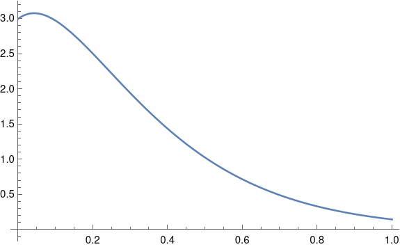
If your purpose is Monte Carlo integration, then yes it is. Our sequence has low discrepancy. You can approximate the integral of a function f over [0, 1] by taking the average of f(xn) over the first N elements of the sequence. Doing Monte Carlo integration with this particular RNG amounts to quasi Monte Carlo (QMC) integration, which is often more efficient than Monte Carlo integration.

Here’s an example using β = e.

    import numpy as np
    
    # Integrate f with N steps of (quasi) Monte Carlo 
    def f(x): return 1 + np.sin(2*np.pi*x)
    N = 1000
    
    # Quasi Monte Carlo
    sum = 0
    x = 0
    e = np.exp(1) 
    for n in range(N):
        sum += f(x)
        x = (x + e) % 1
    print(sum/N)
    
    # Monte Carlo
    sum = 0
    np.random.seed(20220623)
    for _ in range(N):
        sum += f(np.random.random())
    print(sum/N)

This code prints

    0.99901...
    0.99568...

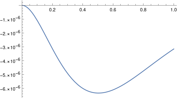
The exact value of the integral is 1, and so the error using QMC between 4 and 5 times smaller than the error using MC. To put it another way, integration using our simple RNG is much more accurate than using the generally better RNG that NumPy uses.

Simulation

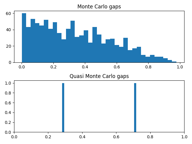
Now suppose we’re doing some sort of simulation that requires computing the gaps between consecutive random numbers. Let’s look at the set of gaps we get using our simple RNG.

    gapset = set()
    x = 0
    for _ in range(N):
        newx = (x + e) % 1
        gap = np.abs(newx - x)
        x = newx
        gapset.add(np.round(gap, 10))
    print( gapset )

Here we rounded the gaps to 10 decimal places so we don’t have minuscule gaps caused by floating point error.

And here’s our output:

    {0.7182818285, 0.2817181715}

There are only two gap sizes! This is a consequence of the three-gap theorem that Greg Egan mentioned on Twitter this morning. Our situation is a slightly different in that we’re looking at gaps between consecutive terms, not the gaps that the interval is divided into. That’s why we have two gaps rather than three.

If we use NumPy’s random number generator, we get 1000 different gap sizes.

Histogram of gap sizes

Cryptography

Random number generators with excellent statistical properties may be completely unsuitable for use in cryptography. A lot of people don’t know this or don’t believe it. I’ve seen examples of insecure encryption systems that use random number generators with good statistical properties but bad cryptographic properties.

These systems violate Kirchhoff’s principle that the security of an encryption system should reside in the key, not in the algorithm. Kirchoff assumed that encryption algorithms will eventually be known, and difficult to change, and so the strength of the system should rely on the keys it uses. At best these algorithms provide security by obscurity: they’re easily breakable knowing the algorithm, but the algorithm is obscure. But these systems may not even provide security by obscurity because it may be possible to infer the algorithm from the output.

Fit for purpose

The random number generator in this post would be terrible for encryption because the sequence is trivially predictable. It would also fail some statistical tests, though it would pass others. It passes at least one statistical test, namely using the sequence for accurate Monte Carlo integration.

Even so, the sequence would pass a one-sided test but not a two-sided test. If you tested whether the sequence, when used in Monte Carlo integration, produced results with error below some threshold, it would pass. But if you looked at the distribution of the integration errors, you’d see that they’re smaller than would be expected from a random sequence. The sequence provides suspiciously good integration results, failing a test of randomness but suggesting the sequence might be useful in numerical integration.

Related posts

Numerically evaluating a theta function

Theta functions pop up throughout pure and applied mathematics. For example, they’re common in analytic number theory, and they’re solutions to the heat equation.

Theta functions are analogous in some ways to trigonometric functions, and like trigonometric functions they satisfy a lot of identities. This post will comment briefly on an identity that makes a particular theta function, θ3, easy to compute numerically. And because there are identities relating the various theta functions, a method for computing θ3 can be used to compute other theta functions.

The function θ3 is defined by

\theta_3(z, t) = 1 + \sum_{k=1}^\infty q^{k^2} \cos(2kz)

where

q = e^{\pi i t}

Here’s a plot of θ3 with t = 1 + i

produced by the following Mathematica code:

    
    q = Exp[Pi I (1 + I)]
    ComplexPlot3D[EllipticTheta[3, z, q], {z, -1, 8.5 + 4 I}]

An important theorem tells us

\theta_3(z, t) = (-it)^{-1/2} \exp(z^2/\pi i t)\, \theta_3\left(\frac{z}{t}, -\frac{1}{t} \right )

This theorem has a lot of interesting consequences, but for our purposes note that the identity has the form

\theta_3(\ldots, t) = \ldots \theta_3\left(\ldots, -\frac{1}{t} \right )

The important thing for numerical purposes is that t is on one side and 1/t is on the other.

Suppose t = a + bi with a > 0 and b > 0. Then

q = \exp\left(\pi i (a + bi)\right) = \exp(-\pi b) \exp(\pi i a)

Now if b is small, |q| is near 1, and the series defining θ3 converges slowly. But if b is large, |q| is very small, and the series converges rapidly.

So if b is large, use the left side of the theorem above to compute the right. But if b is small, use the right side to compute the left.

Related posts

Illegible work

When James Scott uses the word legible, he doesn’t refer to handwriting that is clear enough to read. He uses the word more broadly to mean something that is easy to classify, something that is bureaucrat-friendly. A thing is illegible if it is hard to pigeonhole. I first heard the term from Venkatesh Rao’s essay A Big Little Idea Called Legibility.

Much of the work I do is illegible. If the work were legible, companies would have an employee who does it [1] and they wouldn’t call a consultant.

Here’s a template for a conversation I’ve had a few times:

“We’ve got kind of an unusual problem. It’s related to some things I’ve seen you write about. Have you heard of …?”

“No, what’s that?”

“Never mind. We’d like you to help us with a project. …”

Years ago, when people heard that I worked in statistics they’d ask what programming language I worked in. They expected me to say R or SAS or something like that, but I’d say C++. Not that I recommend doing statistics in C++ [2] in general, but people came to me with unusual projects that they couldn’t get done with standard tools. If an R module would have done what they wanted, they wouldn’t have knocked on my door.

Doing illegible work is a lot of fun, but it’s hard to market. Try typing “Someone who can help with a kinda off the wall math / computer science project” into Google. It’s not helpful. Search engines can only answer questions that are legible to search engines. Illegible work is more likely to come from word of mouth than from a search engine.

***

[1] Sometimes companies call a consultant because they have occasional need for some skill, something they do not need often enough to justify hiring a full-time employee to do. Or maybe they have the skills in house to do a project but don’t have anyone available. Or maybe they want an outside auditor. But in this post I’m focusing on weird projects.

[2] When I mention C++, I know some people are thinking “But isn’t C++ terribly complex?” Why yes, yes it is. But my colleagues and I already knew C++, and we stuck to a sane subset of the language. It was not unusual to rewrite R code in C++ and make it 100x faster.

“Why don’t you just use C?” These days I’m more likely to write C than C++.  Clients don’t want me to write enterprise applications, just small numerical libraries, and they usually ask for C.

Length of periods in the (infinite) periodic table

A few days ago I wrote about what the periodic table would look like if we extended it, assuming the patterns that hold for known elements continue to hold.

That post reported that the number of elements in nth period works out to

 P_n = \frac{(-1)^n(2n+3) + 2n^2 + 6n + 5}{4}

There’s a simpler expression for Pn:

Here ⌊x⌋ is the largest integer no greater than x.

I posted this yesterday on @AlgebraFact. Surely many people have come up with the same formula, but it doesn’t seem to be well known.

Doubly periodic but not analytic

A sine wave is the canonical periodic function, so an obvious way to create a periodic function of two variables would be to multiply two sine waves:

f(x, y) = sin(x) sin(y)

This function is doubly periodic: periodic in the horizontal and vertical directions.

Now suppose you want to construct a doubly periodic function of a complex variable z = x + iy. One thing you might try is

f(x + iy) = sin(x) sin(y)

This is a function of a complex variable, technically, but it’s not what we usually have in mind when we speak of functions of a complex variable. We’re usually interested in complex functions that are differentiable as complex functions.

If h is the increment in the definition of a derivative, we require the limit as h approaches 0 to be equal no matter what route h takes. On the real line, h could go to zero from the left or from the right. That’s all the possibilities. But in the complex plane, h could approach the origin from any angle, or it could take a more complex route such as spiraling toward 0.

It turns out that it is sufficient that the limit be the same whether h goes to 0 along the real or imaginary axis. This gives us the Cauchy-Riemann equations. If

f(x, y) = u(x, y) + i v(x, y)

then the Cauchy-Riemann equations require the partial derivative of u with respect to x to equal the partial derivative of v with respect to y, and the partial derivative of v with respect to x to be the negative of the partial of u with respect to y.

ux = vy
vx = −uy

These equations imply that if v = 0 then u is constant. A real-valued function of a complex variable cannot be analytic unless its constant.

So can we rescue our example by making up an imaginary component v? If so

f(x, y) = sin(x) sin(y) + i v(x, y)

would have to satisfy the Cauchy-Riemann equations. The first equation would require

v(x, y) = − cos(x) cos(y) + a cos(x)

for some constant a, but the second would require

v(x, y) =  cos(x) cos(y) + cos(y)

for some constant b. Note the negative sign in the former but not in the latter. I’ll leave it as an exercise for the reader to show that these requirements are contradictory.

Liouville’s theorem says that a bounded analytic function must be constant. If an analytic function f is doubly periodic, then it must either be constant or have a singularity. There are many such functions, known as elliptic functions.

Related posts

Letter-like Unicode symbols

Unicode provides a way to distinguish symbols that look alike but have different meanings.

We can illustrate this with the following Python code.

    import unicodedata as u

    for pair in [('K', 'K'), ('Ω', 'Ω'), ('ℵ', 'א')]:
        for c in pair:
            print(format(ord(c), '4X'), u.bidirectional(c), u.name(c))

This produces

      4B L LATIN CAPITAL LETTER K
    212A L KELVIN SIGN
     3A9 L GREEK CAPITAL LETTER OMEGA
    2126 L OHM SIGN
    2135 L ALEF SYMBOL
     5D0 R HEBREW LETTER ALEF

Even though K and K look similar, the former is a Roman letter and the latter is a symbol for temperature in Kelvin. Similarly, Ω and Ω are semantically different even though they look alike.

Or rather, they probably look similar. A font may or may not use different glyphs for different code points. The editor I’m using to write this post uses a font that makes no difference between ohm and omega. The letter K and the Kelvin symbol are slightly different if I look very closely. The two alefs appear substantially different.

Note that the mathematical symbol alef is a left-to-right character and the Hebrew latter alef is a right-to-left character. The former could be useful to tell a word processor “This isn’t really a Hebrew letter; it’s a symbol that looks like a Hebrew letter. Don’t change the direction of my text or switch any language-sensitive features like spell checking.”

These letter-like symbols can be used to provide semantic information, but they can also be used to deceive. For example, a malicious website could change a K in a URL to a Kelvin sign.

Related posts

Greek letter paradox

The Greek letter paradox is seeing the same symbol in two contexts and assuming it means the same thing. Maybe it’s used in many contexts, but I first heard it in the context of comparing statistical models.

I used the phrase in my previous post, looking at

α exp(5t) + β t exp(5t)

and

α exp(4.999 t) + β exp(5.001 t).

In both cases, α is the coefficient of a term equal to or approximately equal to exp(5t), so in some sense α means the same thing in both equations. But as that post shows, the value of α depends on its full context. In that sense, it’s a coincidence that the same letter is used in both equations.

When the two functions above are solutions to a differential equation and a tiny perturbation in the same equation, the values of α and β are very different even though the resulting functions are nearly equal (for moderately small t).

Double roots and ODEs

This post will resolve a sort of paradox. The process of solving a difference or differential equation is different when the characteristic equation has a double root. But intuitively there shouldn’t be much difference between having a double root and having two roots very close together.

I’ll first say how double roots effect finding solutions to difference and differential equations, then I’ll focus on the differential equations and look at the difference between a double root and two roots close together.

Double roots

The previous post looked at a second order difference equation and a second order differential equation. Both are solved by analogous techniques. The first step in solving either the difference equation

ayn + byn−1 + cyn−2 = 0

or the differential equation

ay″ + by′ + cy = 0

is to find the roots of the characteristic equation

aλ² + bλ + c = 0.

If there are two distinct roots to the characteristic equation, then each gives rise to an independent solution to the difference or differential equation. The roots may be complex, and that changes the qualitative behavior of the solution, but it doesn’t change the solution process.

But what if the characteristic equation has a double root λ? One solution is found the same way: λn for the difference equation and exp(λt) for the differential equation. We know from general theorems that a second independent solution must exist, but how do we find it?

For the differential equation a second solution is nλn and for the differential equation t exp(λt) is our second solution.

Close roots

For the rest of the post I’ll focus on differential equations, though similar remarks apply to difference equations.

If λ = 5 is a double root of our differential equation then the general solution is

α exp(5t) + β t exp(5t)

for some constants a and b. But if our roots are λ = 4.999 and λ = 5.001 then the general solution is

α exp(4.999 t) + β exp(5.001 t)

Surely these two solutions can’t be that different. If the parameters for the differential equation are empirically determined, can we even tell the difference between a double root and a pair of distinct roots a hair’s breadth apart?

On the other hand, β exp(5t) and β t exp(5t) are quite different for large t. If t = 100, the latter is 100 times larger! However, this bumps up against the Greek letter paradox: assuming that parameters with the same name in two equations mean the same thing. When we apply the same initial conditions to the two solutions above, we get different values of α and β for each, So comparing exp(5t) and t exp(5t) is the wrong comparison. The right comparison is between the solutions to two initial value problems.

We’ll look at two example, one with λ positive and one with λ negative.

Example with λ > 0

If λ > 0, then solutions grow exponentially as t increases. The size of β t exp(λt) will eventually matter, regardless of how small β is. However, any error in the differential equation, such as measurement error in the initial conditions or error in computing the solution numerically, will also grow exponentially. The difference between a double root and two nearby roots may matter less than, say, how accurately the initial conditions are know.

Let’s look at

y″ − 10 y′ + 25 y = 0

and

y″ − 10 y′ + 24.9999 y = 0

both with initial conditions y(0) = 3 and y′(0) = 4.

The characteristic equation for the former has a double root λ = 5 and that of the latter has roots 4.99 and 5.01.

The solution to the first initial value problem is

3 exp(5t) − 11 t exp(5t)

and the solution to the second initial value problem is

551.5 exp(4.99t) − 548.5 exp(5.01t).

Notice that the coefficients are very different, illustrating the Greek letter paradox.

The expressions for the two solutions look different, but they’re indistinguishable for small t, say less than 1. But as t gets larger the solutions diverge. The same would be true if we solved the first equation twice, with y(0) = 3 and y(0) = 3.01.

Example with λ < 0

Now let’s look at

y″ + 10 y′ + 25 y = 0

and

y″ + 10 y′ + 24.9999 y = 0

both with initial conditions y(0) = 3 and y′(0) = 4. Note that the velocity coefficient changed sign from -10 to 10.

Now the characteristic equation of the first differential equation has a double root at -5, and the second has roots -4.99 and -5.01.

The solution to the first initial value problem is

3 exp(−5t)  + 19 t exp(−5t)

and the solution to the second initial value problem is

951.5 exp(−4.99t) − 948.5 exp(5.01t).

Again the written forms of the two solutions look quite different, but their plots are indistinguishable.

Unlike the case λ > 0, now with λ < 0 the difference between the solutions is bounded. Before the solutions started out close together and eventually diverged. Now the solutions are close together forever.

Here’s a plot of the difference between the two solutions.

So the maximum separation between the two solutions occurs somewhere around t = 0.5 where the solutions differ in the sixth decimal place.

Conclusion

Whether the characteristic equation has a double root or two close roots makes a significant difference in the written form of the solution to a differential equation. If the roots are positive, the solutions are initially close together then diverge. If the roots are negative, the solutions are always close together.

More differential equation posts