Another problem with A/B testing: interaction effects

The previous post looked at a paradox with A/B testing: your final result may depend heavily on the order of your tests. This post looks at another problem with A/B testing: the inability to find interaction effects.

Suppose you’re debating between putting a photo of a car or a truck on your website, and you’re debating between whether the vehicle should be red or blue. You decide to use A/B testing, so you test whether customers prefer a red truck or a blue truck. They prefer the blue truck. Then you test whether customers prefer a blue truck or a blue car. They prefer the blue truck.

Maybe customers would prefer a red car best of all, but you didn’t test that option. By testing vehicle type and color separately, you didn’t learn about the interaction of vehicle type and color. As Andrew Gelman and Jennifer Hill put it [1],

Interactions can be important. In practice, inputs that have large main effects also tend to have large interactions with other inputs. (However, small main effects do not preclude the possibility of large interactions.)

Notice that sample size is not the issue. Suppose you tested the red truck against the blue truck with 1000 users and found that 88.2% preferred the blue truck. You can be quite confident that users prefer the blue truck to the red truck. Suppose you also used 1000 users to test the blue truck against the blue car and this time 73.5% preferred the blue truck. Again you can be confident in your results. But you failed to learn something that you might have learned if you’d split 100 users between four options: red truck, blue truck, red car, blue car.

Experiment size

This is an example of a factorial design, testing all combinations of the factors involved. Factorial designs seem impractical because the number of combinations can grow very quickly as the number of factors increases. But if it’s not practical to test all combinations of 10 factors, for example, that doesn’t mean that it’s impractical to test all combinations of two factors, as in the example above. It is often practical to use a full factorial design for a moderate number of factors, and to use a fractional factorial design with more factors.

If you only test one factor at a time, you’re betting that interaction effects don’t matter. Maybe you’re right, and you can optimize your design by optimizing each variable separately. But if you’re wrong, you won’t know.

Agility

The advantage of A/B tests is that they can often be done rapidly. Blue or red? Blue. Car or truck? Truck. Done. Now let’s test something else.

If the only options were between a rapid succession of tests of one factor at a time or one big, complicated statistical test of everything, speed might win. But there’s another possibility: a rapid succession of slightly more sophisticated tests.

Suppose you have 9 factors that you’re interested in, and you understandably don’t want to test several replications of 29 = 512 possibilities. You might start out with a (fractional) factorial design of 5 of the factors. Say that only one of these factors seems to make much difference, no matter what you pair it with. Next you do another experiment testing 5 factors at a time, the winner of the first experiment and the 4 factors you haven’t tested yet. This lets you do two small experiments rather than one big one.

Note that in this example you’re assuming that the factors that didn’t matter in the first experiment wouldn’t have important interactions with the factors in the second experiment. And your assumption might be wrong. But you’re making an educated guess, based on data from the first experiment. This is less than ideal, but it’s better than the alternative of testing every factor one at a time, assuming that no interactions matter. Assuming that some interactions don’t matter, based on data, is better than making a blanket assumption that no interactions matter, based on no data.

Testing more than one factor at a time can be efficient for screening as well as for finding interactions. It can help you narrow in on the variables you need to test more thoroughly.

Related posts

[1] Andrew Gelman and Jennifer Hill. Data Analysis Using Regression and Multilevel/Hierarchical Models. Cambridge University Press, 2007.

A/B testing and a voting paradox

A B testing

One problem with A/B testing is that your results may depend on the order of your tests.

Suppose you’re testing three options: X, Y, and Z. Let’s say you have three market segments, equal in size, each with the following preferences.

Segment 1: X > Y > Z.

Segment 2: Y > ZX.

Segment 3: Z > X > Y.

Now suppose you test X against Y in an A/B test, then test the winner against Z. Segments 1 and 3 prefer X to Y, so X wins the first round of testing. Now you compare X to Z. Segments 2 and 3 prefer Z to X, so Z wins round 2 and is the overall winner.

Now let’s run the tests again in a different order. First we test Y against Z. Segments 1 and 2 will go for Y. Then in the next round, Y against X, segments 1 and 3 prefer X, so X is the overall winner. So one way of running the tests results in Z winning, and another way results in X winning.

Can we arrange our tests so that Y wins? Yes, by testing X against Z first. Z wins the first round, and Y wins in the second round.

The root of the problem is that group preferences are not transitive. We say that preferences are transitive if when someone prefers a to b, and they prefer b to c, then they prefer a to c. We implicitly assumed that each segment has transitive preferences. For example, when we said that the first segment’s preferences are X > Y > Z, we meant that they would rank X > Y,  Y > Z, and X > Z.

Individuals (generally) have transitive preferences, but groups may not. In the example above, the market at a whole prefers X to Y, prefers Y to Z, but prefers Z to X. The segments have transitive preference but the market does not. This is known as the Condorcet voting paradox.

Voting

This is not purely hypothetical. Our example is simplified, but it reflects a phenomenon that does happen in practice. It has been observed in voting. Constituencies in a legislature may have transitive preferences while the legislature as a whole does not. This opens the possibility of manipulating the final outcome by controlling the order in which items are voted on. In the example above, someone who knows the preferences of the groups could make any of the three outcomes the winner by picking the order of A/B comparisons.

Political scientists have looked back at congressional voting records and found instances of this happening, and can roughly determine when someone first discovered the technique of rigging sequential votes. They can also roughly point to when legislators became aware of the manipulation and learned that they sometimes need to vote against their actual preferences in one vote in order to get a better outcome at the end of the sequence of votes. (I think this was around 1940, but my memory could be wrong.) Political scientists call this sophisticated voting, as opposed to naive voting in which one always votes according to honest preferences.

Market research

The voting example is relevant to market research because it shows that intransitive group preferences really happen. But unlike in voting, customers respond honestly to A/B tests. They don’t even know that they’re part of an A/B test.

In the example above, we come away from our test believing that we have a clear winner. In both rounds of testing, the winner gets twice as many responses as the loser. The large margin in each test is misleading.

Any of the three options could be the winner, depending on the order of testing, but none of the options is any better than the others. So in the example we don’t so much make a bad choice, but we have too much confidence in our choice.

But now suppose the groups are not all the same size. Suppose the three segments represent 45%, 35%, and 20% of the market respectively. We can still have any option be the final winner, depending on the order of testing. But now some rests are better than others. If we tested all three options at once in an A/B/C test, we’d learn that a plurality of the market prefers X, and we’d learn that there is no option that the market as a whole prefers.

Related posts

Smoothly extending arctan(k tan(t))

I wrote a while back about the function

f(t) = arctan(k tan(t)).

I keep running into this function. Has anybody given this function a name or studied it?

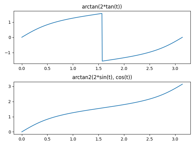
The direct implementation has a discontinuity at π/2 but I needed to extend it continuously. Using the two-argument version of inverse tangent fixes this. In Python, the implementation is

    arctan2(k*sin(t), cos(t))

Here are plots of the direct and improved version.

Mathematica does not have a function ArcTan2. Instead, it overloads the ArcTan function to take either one or two arguments. But beware: the two-argument version of ArcTan in Mathematica takes its arguments in the opposite order of functions like atan2 in C.

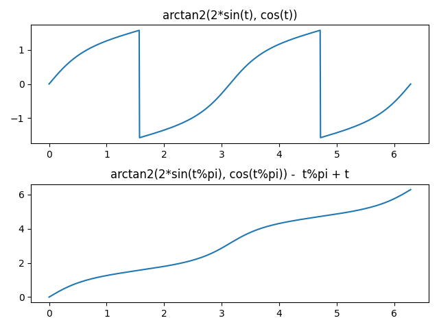
This extends the continuous range from [0, π/2] to [0, π], but there’s still a discontinuity at π. The trick to extending further is to reduce the argument mod π, subtract off the reduced argument, then add the original argument back in. In Python:

    arctan2(k*sin(t%pi), cos(t%pi)) - t%pi + t

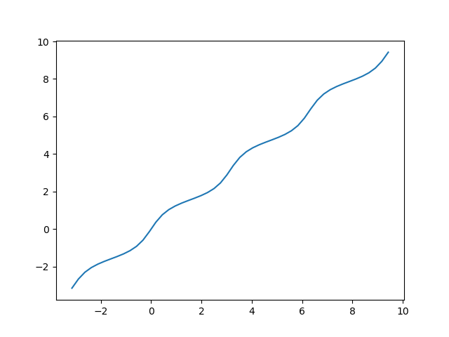
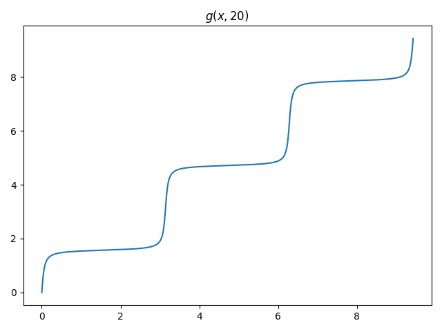
This plot shows the extension works.

Now the function extends smoothly to the entire real line.

Here’s a Mathematica implementation of the smooth extension.

    g[x_, k_] := Module[{y = Mod[x, Pi]}, ArcTan[Cos[y], k Sin[y]] - y + x]

The function g(x, k) is an increasing function of x for fixed k ≠ 0, and its inverse is the same function replacing k with 1/k:

g( g(x, 1/k), k ) = x.

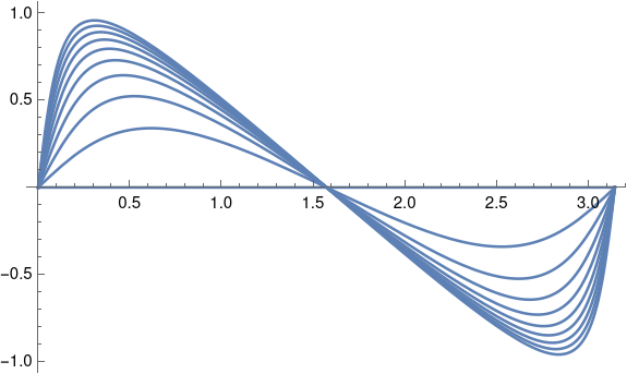
Here’s a plot of the function g with the linear trend subtracted, letting k vary from 1 to 10.

This was made with the following code.

    Plot[Table[g[x, n] - x, {n, 1, 10}], {x, 0, Pi}]

As k increases, the amplitude increases, and the peaks move away from the center. You can confirm this by taking the derivative. The maximum occurs at arccos(√(k/(k+1))) and so the maxima locations converge to 0 as k → ∞. By symmetry the minima locations converge to π.You can also verify that the maximum value is arctan(√k), and so the maxima converge to π/2, and by symmetry the minima converge to -π/2;.

This plot looks similar to the plot of true anomaly for a highly elliptical orbit. I’m sure they’re related, but I haven’t worked out exactly how.

If we add back in the linear trend that we’d subtracted off, we see that for large k, g(x, k) is a smooth approximation to a stairstep function, analogous to the soft maximum function.

Related posts

Random illustrations of Pascal’s theorem

Pascal’s theorem begins by selecting any six distinct points on an ellipse and drawing a “hexagon.” I put hexagon in quotes because the result need not look anything like a hex nut. In this context it simply means to pick one point, connect it to some other point, and so forth, joining the points in a cycle. The points need not be in order around the ellipse, and so the hexagon can, and usually will, be irregularly shaped.

Pascal’s theorem says that the intersections of opposite sides intersect in three points that lie in on a common line. Since the hexagon can be irregularly shaped, it’s not immediately clear what the “opposite” sides are.

The segment joining points 1 and 2 is opposite the segment joining points 4 and 5. The segment joining points 2 and 3 is opposite the segment joining points 5 and 6.The segment joining points 3 and 4 is opposite the segment joining points 6 and 1. If the hexagon were a regular hexagon, opposite sides would be parallel.

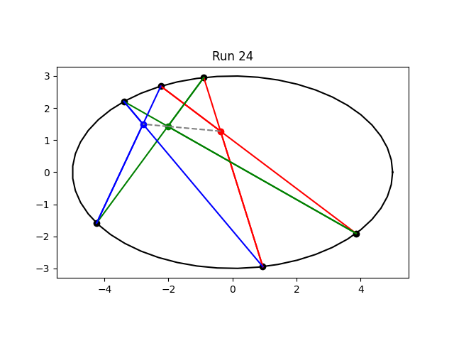
The theorem is usually illustrated with something like the figure below.

Opposite sides share the same color. The blue, green, and red dots inside the ellipse are the intersections of the blue sides, the green sides, and the red sides respectively. And as Pascal predicted, the three points are colinear.

The statement of Pascal’s theorem above is incomplete. We have to look at where the lines containing the sides intersect, not where the sides intersect. In the image above, the lines intersect where the line segments intersect, but this doesn’t always happen.

The Wikipedia article on Pascal’s theorem says “the three pairs of opposite sides of the hexagon (extended if necessary) meet at three points which lie on a straight line.” The parenthetical remark to extend the sides “if necessary” could lead you to think that needing to extend the sides is the exceptional case. It’s not; it’s the typical case.

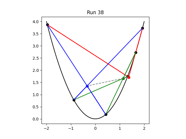
The graph above is typical of presentations of Pascal’s theorem, but not typical of randomly selected points on an ellipse. I wrote a program to select random points on an ellipse and connect them as the theorem requires. The title of the plot above is “Run 24” because that was the first run to produce a typical illustration.

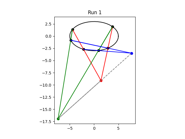
Here’s what the first run looked like.

In this example, all three intersection points are outside the ellipse. It’s hard to see the blue side on the bottom of the ellipse; it’s so short that the ellipse is practically flat over that distance and the blue line lies nearly on top of the black arc of the ellipse. This is a more typical example: usually one or more intersection points lies outside the ellipse, and usually one or more sides is hard to see.

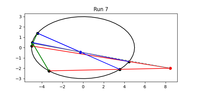
Here’s an example that is even more typical.

Seeing this kind of plot first make me think there was a bug in my program. The shorter green side is hard to see, the intersection of the two green lines is lost between two points clumped close together, and the gray line connecting the three intersection points lies practically on top of a couple other lines.

Random examples and random tests

Random examples are complementary to clean classroom examples. The first image, Run 24, is typical in presentations for good reasons: it’s easy to see all the sides, and all the action happens in a small area. But random examples give you a better appreciation for the range of possibilities. This is very similar to software testing: some tests should be carefully designed and some should be chosen at random.

Conic sections

Pascal’s theorem applies to conic sections in general, not just ellipses. Here is an example with a parabola.

Randomly selected examples for parabolas are even less legible than random examples for ellipses. It’s common for lines to pile up on top of each other.

Projective geometry

Strictly speaking Pascal’s theorem is a theorem in projective geometry. It tacitly assumes that the lines in question do intersect. In the Euclidean plane two of the sides might be parallel and not intersect. In projective geometry parallel lines intersect “at infinity.” Or rather, there are no parallel lines in projective geometry.

With randomly selected points, the probability of two lines being parallel is 0. But it is possible that two lines are nearly parallel and intersect far from the ellipse. Some of the runs I made for this post did just this, like Run 9 below.

If you’ve got room for one illustration, you’d naturally use something like Run 24, but it’s good to know that things like Run 9 can happen too.

Related posts

Finding where two quadratic curves intersect

Suppose you have two quadratic polynomials in two real variables, f(x, y) and g(x, y), and you want to know whether the two curves

f(x, y) = 0

and

g(x, y) = 0

intersect, and if they do, find where they intersect.

David Eberly has a set of notes on solving systems of polynomial equations that give the conditions you need. The conditions are quite complicated, but they are explicit and do not involve any advanced math. He gives 14 equations that combine to form the coefficients in a 4th degree polynomial that will tell you whether the curves intersect, and will get you started on finding the points of intersection.

Algebraic geometry

There is a more elegant solution, but it requires much more background. It requires working in the complex projective plane ℙ² rather than the real plane ℝ². What does that mean? First, it means you work with complex numbers rather than real numbers. Second, it means adding “points at infinity.” This sounds awfully hand-wavy, but it can all be made rigorous using homogeneous coordinates with three complex numbers.

If you haven’t seen this before, you may be thinking “You want me to go from pairs of real numbers to triples of complex numbers? And this is supposed to make things easier?!” Yes, it actually does make things easier.

Once you move to ℙ², the question of whether the curves f(x, y) = 0 and g(x, y) = 0 intersect becomes trivial: yes, they intersect. Always. A special case of Bézout’s theorem says any two quadratic curves are either the same curve or they intersect in at 4 points, counting intersections with multiplicity.

Your original question was whether the curves intersect in ℝ², and now that question reduces to asking whether the 4 points guaranteed by Bézout’s theorem lie in ℝ². They might not be real, or they might be points at infinity.

Even if you go by David Eberly’s more elementary approach, you still face a similar question. You have a fourth degree polynomial, and you need to know whether it has real roots. How would you do that? You’d probably find all four complex roots first and see whether any are in fact real. Moving from the real numbers to the complex numbers makes it easier to find the roots of polynomials, and moving to complex projective space carries this idea further.

In the real plane ℝ² the zero set of a quadratic polynomial can be an ellipse, a parabola, or a hyperbola. (The circle is a special case of an ellipse.) But in ℙ² there is only one kind of conic section: there is a change of variables that turns the zero set of any quadratic polynomial into a circle. So now we’ve reduced the problem to finding where two circles intersect.

Finding the intersection of two conic sections illustrates the principles discussed in the preface to Algebraic Geometry: A Problem Solving Approach.

One way of doing mathematics is to ask bold questions about the concepts your are interested in studying. Usually this leads to fairly complicated answers having many special cases. An important advantage to his approach is that questions are natural and easy to understand. A disadvantage is that proofs are hard and often involve clever tricks, the origins of which are very hard to see.

A second approach is to spend time carefully defining the basic terms, with the aim that the eventual theorems and proofs are straightforward. Here the difficulty is in understanding how the definitions, which often initially seem somewhat arbitrary, ever came to be. The payoff is that the deep theorems are more natural, their insights more accessible, and the theory made more aesthetically pleasing.

Related posts


A more convenient squircle equation

A few years ago I wrote several posts about “squircles”, starting with this post. These are shapes satisfying

|x|^p + |y|^p = 1

where typically p = 4 or 5. The advantage of a squircle over a square with rounded edges is that the curvature varies continuously around the figure rather than jumping from a constant positive value to zero.

Manuel Fernández-Guasti developed a slightly different shape also called a squircle but with a different equation

x^2 + y^2 = s^2 x^2 y^2 + 1

We need to give separate names to the two things called squircles, and so I’ll name them after their parameters: p-squircles and s-squircles.

As s varies from 0 to 1, s-squircles change continuously from a circle to a square, just as p-squircles varies do as p goes from 2 to ∞.

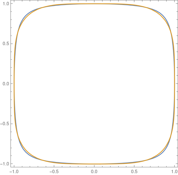
The two kinds of squircles are very similar. Here’s a plot of one on top of the other. I’ll go into detail later of how this plot was made.


Advantage of s-squircles

The equation for a p-squircle is polynomial if p is an even integer, but in general the equation is transcendental. The equation for an s-squircle is a polynomial of degree 4 for all values of s. It’s more mathematically convenient, and more computationally efficient, to have real numbers as coefficients than as exponents. The s-squircle is an algebraic variety, the level set of a polynomial, and so can be studied via algebraic geometry whereas p-squircles cannot (unless p is an even integer).

It’s remarkable that the two kinds of squircles are so different in the structure of their defining equation and yet so quantitatively close together.

Equal area comparison

I wanted to compare the two shapes, so I plotted p-squircles and s-squircles of the same area.

The area of a p-squircle is given here where n = 2. The area of an s-squircle is given here MathWorld where k = 1.

\begin{align*} A_1(p) &= 4\, \frac{\Gamma\left(1 + \frac{1}{p} \right )^2}{\Gamma\left(1 + \frac{2}{p} \right )} \\ A_2(s) &= 4\, \frac{E(\sin^{-1}s, s^{-1})}{s} \end{align*}

Here E is the “elliptic integral of the second kind.” This function has come up several times on the blog, for example here.

Both area function are increasing functions of their parameters. We have A1(2) = A2(0) and A1(∞) = A2(1). So we can pick a value of p and solve for the corresponding value of s that gives the same area, or vice versa.

The function A1 can be implemented in Mathematica as

    A1[p_] := 4 Gamma[1 + 1/p]^2/Gamma[1 + 2/p]

The function A2 is little trickier because Mathematica parameterizes the elliptic integral slightly differently than does the equation above.

    A2[s_] := 4 EllipticE[ArcSin[s], s^-2]/s

Now I can solve for the values of s that give the same area as p = 4 and p = 5.

    FindRoot[A2[s] == A1[4], {s, 0.9}]

returns 0.927713 and

    FindRoot[A2[s] == A1[5], {s, 0.9}]

returns 0.960333. (The 0.9 argument in the commands above is an initial guess at the root.)

The command

    ContourPlot[{x^2 + y^2 == 0.927713 ^2 x^2 y^2 + 1, 
        x^4 + y^4 == 1}, {x, -1, 1}, {y, -1, 1}]

produces the following plot. This is the same plot as at the top of the post, but enlarged to show detail.

The command

    ContourPlot[{x^2 + y^2 == 0.960333 ^2 x^2 y^2 + 1, 
        Abs[x]^5 + Abs[y]^5 == 1}, {x, -1, 1}, {y, -1, 1}]

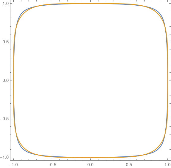
produces this plot

In both cases the s-squircle is plotted in blue, and the p-squircle in gold. The gold virtually overwrites the blue. You have to look carefully to see a little bit of blue sticking out in the corners. The two squircles are essentially the same to within the thickness of the plotting lines.

History

The term “squircle” goes back to 1953, but was first used as it is used here around 1966. More on this here.

However, Fernández-Guasti was the first to use the term in scholarly literature in 2005. See the discussion in the MathWorld article.

Determining a conic by points and tangents

The first post this series said that a conic section has five degrees of freedom, and that any theorem that claims to determine a conic by less than five numbers is using some additional implicit information.

The second post looked at Gibbs’ method which uses three observations, and a variation on the method uses just one observation. The post explains where the missing information is hiding.

The third post looked at Lambert’s theorem which determines a conic section from two observations and again explains where the additional information comes from.

You could also determine a conic by an assortment of points and tangent lines (physically, a set of observations and velocities). You could specify four points on the conic and a line it must be tangent to. Or you could specify three points and two tangents, etc. See, for example, here.

As a general rule, any five reasonable pieces of information about a conic section are enough to determine it uniquely. The tedious part is writing down the exceptions to the general rule. For example, you can’t have three of the points lie on a line.

You can’t always get by with saying “I’ve got n degrees of freedom and n pieces of information, so there must be a solution.” And yet remarkably often you can.

Lambert’s theorem

At the start of this series we pointed out that a conic section has five degrees of freedom, and so claims to be able to determine an orbit from less than five numbers must be hiding information somewhere. That is the case with Lambert’s theorem which reportedly determines an orbit from two numbers.

Lambert’s theorem says that the time between two observations of an object in an elliptical orbit can be determined by the sum of the distances to the two observations, the length of the chord connecting the two observations, and the semi-major axis of the ellipse. From this one can determine the equation of the ellipse.

Let r1 be the distance to the first observation and r2 the distance to the second observation, and C the length of the chord between the two observations. We don’t need to know r1 and r2 individually but only their sum r1 + r2. And if we know the angle between the two observations we can use the law of cosines to find C. However we get there, we have two lengths: r1 + r2 and C. We also know a, the length of the semi-major axis. This gives us three lengths.

The observations are taken from the body being orbited, so we implicitly know one of the foci of the ellipse. That’s four pieces of information. The fifth is the mass of the object being orbited.

Lambert’s theorem divides into three cases: elliptic, parabolic, and hyperbolic.

Elliptical orbits

For an object in an elliptic orbit, Lambert’s theorem becomes

\sqrt{\frac{\mu}{a^3}} (t_2 - t_1) = \alpha - \beta - (\sin \alpha - \sin\beta)

where μ is the standard gravitational parameter, equal to GM where G is the gravitational constant and M is the mass of the body orbited. The angles α and β are given by

 \begin{align*} \sin\frac{\alpha}{2} = \frac{1}{2}\left( \frac{r_1 + r_2 + C}{a} \right)^{1/2} \\ \sin\frac{\beta}{2} = \frac{1}{2}\left( \frac{r_1 + r_2 - C}{a} \right)^{1/2} \\ \end{align*}

Hyperbolic orbits

The hyperbolic case is very similar, replacing sine with hyperbolic sine.

\sqrt{\frac{\mu}{a^3}} (t_2 - t_1) = \gamma - \delta - (\sin \gamma - \sin\delta)

where

\begin{align*} \sinh\frac{\gamma}{2} = \frac{1}{2}\left( \frac{r_1 + r_2 + C}{a} \right)^{1/2} \\ \sinh\frac{\delta}{2} = \frac{1}{2}\left( \frac{r_1 + r_2 - C}{a} \right)^{1/2} \\ \end{align*}

Parabolic orbits

The parabolic case was worked out by Newton:

t_2 - t_1 = \frac{1}{6\sqrt{mu}}\left( (r_1 + r_2 + C)^{3/2} - (r_1 + r_2 - C)^{3/2}\right)

Other posts in this series

Source: Adventures in Celestial Mechanics by Victor Szebehely

Gibbs’ method of determining an orbit

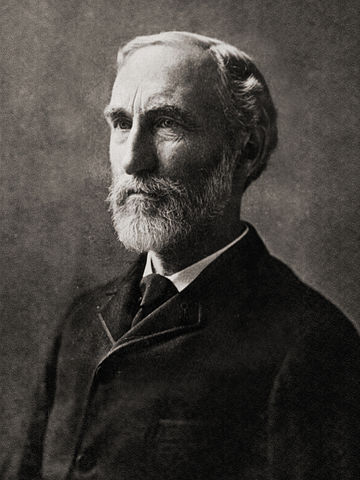
Josiah Willard Gibbs

Josiah Willard Gibbs (1839–1903) was prominent American scientist at a time when America had yet to produce many prominent scientists. I first heard of him via Gibbs phenomenon and later by attending one of the Gibbs lectures at an AMS meeting.

Gibbs came up with a method of determining an orbit from three observations. As discussed earlier, a conic section has five degrees of freedom. So how can we determine a conic section, i.e. a two-body problem orbit, from three observations?

Mars Orbiter

As a warm-up to Gibbs’ method, let’s look back at the post on India’s Mars Orbiter Mission. There we determined an orbit by just two observations. What determined the missing three degrees of freedom?

The post on the Mars Orbiter Mission (MOM) didn’t use two arbitrary observations but two very special observations, namely the nearest and furthest approaches of the probe. Because the distances were known relative to Mars, we know the position of one of the foci of the orbit, i.e. the center of mass of Mars. And because the two observations are on opposite sides of the orbit, we know where the other focus is. And because these observations were along the major axis of the ellipse, we know the orientation of the ellipse. All together we know five facts about the orbit.

Gibbsian method

Gibbs method starts with three facts about the orbit, the position of a satellite at three points in its orbit. These are not simply three points on the ellipse but three measurements taken from the body that the satellite is orbiting. That means we know the position of one of the foci, i.e. the body being orbited. Gibbs’ method also assumes we know the mass of body being orbited, so that’s our fifth piece of information.

So with the Mars Orbiter Mission we had two special observations. The “specialness” of these observations provided two more pieces of data, and the fact that the measurements were taken from a focus of the orbit gave us the fifth piece of information.

With Gibbs’ method, we have an extra observation, but none of the observations are special. So we’re up one piece of information from observation but down two pieces of information related to specialness. The missing piece of information is supplied by a physical quantity, the mass of the object orbited.

Radar observation

There is a variation on Gibbs’ method that uses only one observation. It is based on radar observation, not optical observation, and includes the velocity of the object as well as its position. So two partial derivatives, rates of change in two perpendicular directions, replace two of the observations. We still need five bits of information to determine five degrees of freedom.

Preliminary determination

The methods this series of posts use the minimum amount of information algebraically necessary to determine an orbit. In practice, these methods are used for preliminary orbit determination, i.e. they give an approximate result that could be bootstrapped to obtain a more accurate solution.

Under ideal circumstances more further observations would be redundant, but in practice having more observations lets measurement errors cancel each other out to some extent. This observation was a milestone in the development of modern statistics: the problem of determining orbits from multiple observations lead to regression theory.

Notes

You can find the details of how to determine an orbit from three observations in Fundamentals of Astrodynamics by Bate, Mueller, and White. The book also covers determining an orbit from one radar observation with derivatives.

The next post in this series looks at Lambert’s theorem for determining an orbit from two observations (plus three other pieces of information).