Mathematical stability vs numerical stability

Is 0 a stable fixed point of f(x) = 4x (1-x)?

If you set x = 0 and compute f(x) you will get exactly 0. Apply f a thousand times and you’ll never get anything but zero.

But this does not mean 0 is a stable attractor, and in fact it is not stable.

It’s easy to get mathematical stability and numerical stability confused, because the latter often illustrates the former. In this post I point out that the points on a particular unstable orbit cannot be represented exactly in floating point numbers, so iterations that start at the floating  point representations of these points will drift away.

In the example here, 0 can be represented exactly, and so we do have a computationally stable fixed point. But 0 is not a stable fixed point in the mathematical sense. Any starting point close to 0 but not exactly 0 will eventually go all over the place.

If we start at some very small ε > 0, then f(ε) ≈ 4ε. Every iteration multiplies the result by approximately 4, and eventually the result is large enough that the approximation no longer holds.

For example, suppose we start with x = 10-100. After 100 iterations we have

x = 4100 10-100 = 1.6 × 10-40.

If we were to plot this, we wouldn’t see any movement. But by the time we iterate our function 200 times, the result is chaotic. I get the following:

Spaceship operator in Python

Some programming languages, such as Perl, have an infix operator <=> that returns a three-state comparison. The expression

    a <=> b

evaluates to -1, 0, or 1 depending on whether a < b, a = b, or a > b. You could think of <=> as a concatenation of <, =, and >.

The <=> operator is often called the “spaceship operator” because it looks like Darth Vader’s ship in Star Wars.

Python doesn’t have a spaceship operator, but you can get the same effect with numpy.sign(a-b). For example, suppose you wanted to write a program to compare two integers.

You could write

    from numpy import sign
    def compare(x, y):
        cmp = ["equal to", "greater than", "less than"][sign(x-y)]
        print(f"{x} is {cmp} {y}.")

Here we take advantage of the fact that an index of -1 points to the last element of a list.

The sign function will return an integer if its argument is an integer or a float if its argument is a float. The code above will break if you pass in floating point numbers because sign will return -1.0, 0.0, or 1.0. But if you replace sign(x-y) with int(sign(x-y)) it will work for floating point arguments.

Related post: Symbol pronunciation

Real radical roots

The previous post Does chaos imply period 3? ended with looking at a couple cubic polynomials whose roots have period 3 under the mapping f(x) = 4x(1-x). These are

64 x³ – 112 x² + 56 x – 7

and

64 x³ – 96 x² + 36 x – 3.

I ended the post by saying you could find their roots numerically using the NSolve function in Mathematica.

What if you wanted to find the roots exactly? You could try using the NSolve function rather than the NSolve solve function, but you won’t get anything back. Doesn’t Mathematica know how to solve a cubic equation? Yes it does, and you can force it to use the cubic equation by using the ToRadicals function.

If you apply ToRadicals to the roots, Mathematica will give you the roots in radical form, with expressions involving complex numbers. For example, here’s the smallest root of the first polynomial:

 x = \frac{7}{12} -\frac { 7^{2/3} \left(1+i\sqrt{3}\right) }{ 12\ 2^{2/3} \sqrt[3]{-1+3 i \sqrt{3}} } -\frac{1}{24} \left(1-i \sqrt{3}\right) \sqrt[3]{ \frac{7}{2} \left(-1+3 i \sqrt{3}\right)}

But the roots of these polynomials are clearly real as you can see from their graphs.

.

If we didn’t have access to a graph, we could show that the roots are real and distinct by computing the discriminant and seeing that it is positive.

Casus irreducibilis

The polynomials have degree less than 5, so their roots can be expressed in terms of radicals. And the roots are real. But they cannot be expressed in terms of real radicals!

This an example of the “casus irreducibilis.” Most cubic equations with real roots cannot be solved using real radicals. The casus irreducibilis theorem says that the roots of a cubic polynomial can be written in terms of real radicals if and only if one of the roots is rational.

This says there’s a sort of excluded middle ground: the roots cannot involve cubic roots with real numbers. They are either simpler or more complex. If there is a rational root, you can factor it out and find the other two roots with the quadratic equation, i.e. only using square roots, not cubic roots. But if there is no rational root, expressing the roots in terms of radicals requires cube roots and complex numbers.

Our polynomials

The rational root test says that if a polynomial has a rational root p/q then q must be a factor of the leading coefficient and p must be a factor of the constant term. So in our first cubic

64 x³ – 112 x² + 56 x – 7

any rational root must have denominator 1, 2, 4, …, 64 and numerator either 1 or 7. We can check all the possibilities and see that none of them are zeros.

Similarly the only possible rational roots of

64 x³ – 96 x² + 36 x – 3

must have denominator 1, 2, 4, …, 64 and numerator either 1 or 3, and none of them are zeros.

So the roots of our cubic polynomials can be expressed in terms of radicals, but not without complex numbers, even though the roots are all real.

Unstable orbit

The reason we were interested in these two polynomials is that we were looking for orbits of period 3 under iterations of 4x(1-x). And we found them. But they form an unstable orbit.

If we make a cobweb plot of the iterations starting at any one of the roots, it appears that multiple applications of 4x(1-x) just rotate between the three roots.

But with a few more iterations—the plot below shows 100 iterations—we can see that these points are not stable. Unless you start exactly on one of the roots, which you cannot since they’re irrational, you will wander away from them.

Does chaos imply period 3?

Sharkovskii’s theorem says that if a continuous map f from an interval I to itself has a point with period 3, then it has a point with period 5. And if it has a point with period 5, then it has points with order 7, etc. The theorem has a chain of implications that all begins with 3. If you have points with period 3, you have points of all periods.

Now suppose you want to go “upstream” in Sharkovskii’s chain of implications. If you have a point with period 5, do you have a point with period 3? The answer is no: a map can have points with period 5 without having points of period 3, though it necessarily has points with all other positive integer periods except 3.

There’s an example illustrating the claim above that I’ve seen in multiple places, but I haven’t seen it presented graphically. You could work through the example analytically, but here I present it graphically.

This is the example function written in Python.

    def f(x):
        assert(1 <= x <= 5)
    
        if x < 2:
            return 1 + 2*x
        if x < 3:
            return 7 - x
        if x < 4:
            return 10 - 2*x
        if x <= 5:
            return 6 - x

Here’s a graphical demonstration that f has a fixed point, but no points of period 3.

The only point fixed under applying f three times is the point that was already fixed under applying f once.

This graph shows that f has points with period 5:

By Sharkovskii’s theorem f must have points with all other periods, except 3. Here’s a demonstration that it has points with period 6.

The map f is chaotic, but it does not have a point with period 3.

Logistic map

Let’s look at the most famous chaotic map, the logistic map.

f(x) = rx (1 – x)

where x is in [0, 1] and r is in [0. 4].

logistic bifurcation diagram

The images above shows orbits as r ranges over [0, 4]. Clearly f has points with period 2. There’s a whole interval of values of r that lead to points with period 2, roughly for r between 3 and 3.5. And we can see for r a little bigger there are points of period 4. But is there any point with period 3?

We can look for points of period 3 at the end of the plot, where r = 4, using Mathematica.

Define

    f[x_] := 4 x (1 - x)

and look for points where f³(x) = x using

    Factor[f[f[f[x]]] - x]

This shows that the solutions are the roots of

x (-3 + 4 x) (-7 + 56x – 112x² + 64 x³) (-3 + 36x – 96x² + 64x³)

The first two roots are fixed points, points of period 1, but the roots of the two cubic factors are points with period 3.

The cubics clearly have all their roots in the interval [0,1] and we could find their numerical values with

    NSolve[f[f[f[x]]] == x, x]

Although the roots are fixed points, they are unstable fixed points, as demonstrated at the bottom the next post.

Related posts

Sarkovsky’s theorem

The previous post explained what is meant by period three implies chaos. This post is a follow-on that looks at Sarkovsky’s theorem, which is mostly a generalization of that theorem, but not entirely [1].

First of all, Mr. Sarkovsky is variously known Sharkovsky, Sharkovskii, etc. As with many Slavic names, his name can be anglicized multiple ways. You might use the regular expression Sh?arkovsk(ii|y) in a search.

The theorem in the previous post, by Li and Yorke, says that if a continuous function from a closed interval to itself has a point with period three, it has points with all positive periods. This was published in 1975.

Unbeknownst to Li and Yorke, and everyone else in the West at the time, Sarkovsky had published a more general result in 1964 in a Ukrainian journal. He demonstrated a total order on the positive integers so that the existence of a point with a given period implies the existence of points with all periods further down the sequence. The sequence starts with 3, and every other positive integer is in the sequence somewhere, so period 3 implies the rest.

Sarkivsky showed that period 3 implies period 5, period 5 implies period 7, period 7 implies period 9, etc. If a continuous map of an interval to itself has a point of odd period n > 1, it has points with order given by all odd numbers larger than n. That is, Sarkovsky’s order starts out

3 > 5 > 7 > …

The sequence continues

… 2×3 > 2×5 > 2×7 > …

then

… 2²×3 > 2²×5 > 2²×7 > …

then

… 2³×3 > 2³×5 > 2³×7 > …

and so on for all powers of 2 times odd numbers greater than 1.

The sequence ends with the powers of 2 in reverse order

… 2³ > 2² > 1.

Here’s Python code to determine whether period m implies period n, assuming m and n are not equal.

from sympy import factorint

# Return whether m comes befor n in Sarkovsky order
def before(m, n):

    assert(m != n)

    if m == 1 or n == 1:
        return m > n

    m_factors = factorint(m)
    n_factors = factorint(n)

    m_odd = 2 not in m_factors
    n_odd = 2 not in n_factors
    
    m_power_of_2 = len(m_factors) == 1 and not m_odd
    n_power_of_2 = len(n_factors) == 1 and not n_odd

    if m_odd:
        return m < n if n_odd else True if m_power_of_2: return m > n if n_power_of_2 else False

    # m is even and not a power of 2    
    if n_odd:
        return False
    if n_power_of_2:
        return True
    if m_factors[2] < n_factors[2]: return True if m_factors[2] > n_factors[2]:
        return False  
    return m < n

Next post: Can you swim “upstream” in Sarkovsky’s order?

[1] There are two parts to the paper of Li and Yorke. First, that period three implies all other periods. This is a very special case of Sarkovsky’s theorem. But Li and Yorke also proved that period three implies an uncountable number of non-periodic points, which is not part of Sarkovsky’s paper.

Period three implies chaos

One of the most famous theorems in chaos theory, maybe the most famous, is that “period three implies chaos.” This compact statement comes from the title of a paper [1] by the same name. But what does it mean?

This post will look at what the statement means, and the next post will look at a generalization.

Period

First of all, the theorem refers to period in the sense of function iterations, not in the sense of translations. And it applies to particular points, not to the function as a whole.

The sine function is periodic in the sense that it doesn’t change if you shift it by 2π. That is,

sin(2π+x) = sin(x)

for all x. The sine function has period 2π in the sense of translations.

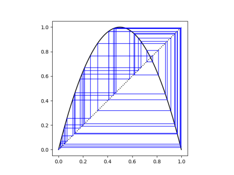
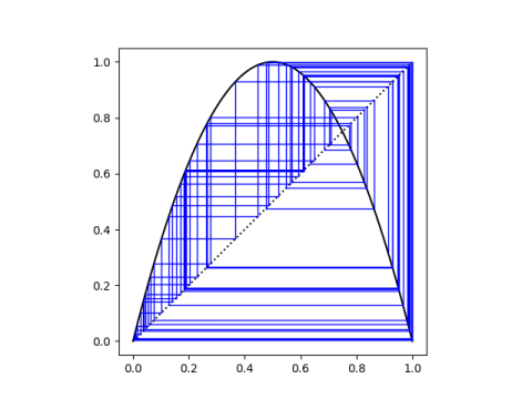
In dynamical systems, period refers to getting the same result, not when you shift a function, but when you apply it to itself. A point x has period n under a function f if applying the function n times gives you x back, but applying it any less than n times does not.

So, for example, the function f(x) = –x has period 2 for non-zero x, and period 1 for x = 0.

Three

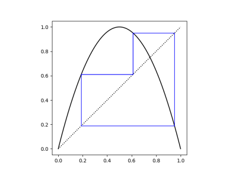
Period three specifically means

f( f( f(x) ) ) = x

but

xf(x)

and

xf( f(x) ).

Note that this is a property of x, not a property of f per se. That is, it is a property of f that one such x exists, but it’s not true of all points.

In fact it’s necessarily far from true for all points, which leads to what we mean by chaos.

Chaos

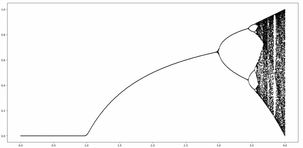
If f is a continuous function from some interval I to itself, it cannot be the case that all points have period 3.

If one point has period 3, then some other point must have period 4. And another point must have period 97. And some point has period 1776.

If some point in I has period 3, then there are points in I that have period n for all positive n. Buy one, get infinitely many for free.

And there are some points that are not periodic, but every point in I is arbitrarily close to a point that is periodic. That is, the periodic points are dense in the interval. That is what is meant by chaos [2].

This is really an amazing theorem. It says that if there is one point that satisfies a simple condition (period three) then the function as a whole must have very complicated behavior as far as iteration is concerned.

More

If the existence of a point with period 3 implies the existence of points with every other period, what can you say about, for example, period 10? That’s the subject of the next post.

More posts on dynamical systems and chaos.

[1] Li, T.Y.; Yorke, J.A. (1975). “Period Three Implies Chaos” American Mathematical Monthly. 82 (10): 985–92.

[2] There is no single definition of chaos. Some take the existence of dense periodic orbits as the defining characteristic of a chaotic system. See, for example, [3].

[3] Bernd Aulbach and Bernd Kieninger. On Three Definitions of Chaos. Nonlinear Dynamics and Systems Theory, 1(1) (2001) 23–37

Better approximation for ln, still doable by hand

A while back I presented a very simple algorithm for computing natural logs:

log(x) ≈ (2x – 2)/(x + 1)

for x between exp(-0.5) and exp(0.5). It’s accurate enough for quick mental estimates.

I recently found an approximation by Ronald Doerfler that is a little more complicated but much more accurate:

log(x) ≈ 6(x – 1)/(x + 1 + 4√x)

for x in the same range. This comes from Doerfler’s book Dead Reckoning.

It requires calculating a square root, and in exchange for this complication gives about three orders of magnitude better approximation. You could use it, for example, on a calculator that has a square root key but not log key. Or if you’re dead reckoning, you need to take a square root by hand.

Here’s a plot of the error for both approximations.

The simpler approximation has error about 10-2 on each end, whereas Doerfler’s algorithm has error about 10-5 on each end.

If you can reduce your range to [-1/√2, √2] by pulling out powers of 2 first and remembering the value of log(2), then Doerfler’s algorithm is about six times more accurate.

By the way, you might wonder where Doerfler’s approximation comes from. It’s not recognizable as, say, a series expansion. It comes from doing Richardson extrapolation, but algebraically simplified rather than expressing it as an algorithm.

Beta distribution with given mean and variance

It occurred to me recently that a problem I solved numerically years ago could be solved analytically, the problem of determining beta distribution parameters so that the distribution has a specified mean and variance. The calculation turns out to be fairly simple. Maybe someone has done it before.

Problem statement

The beta distribution has two positive parameters, a and b, and has probability density proportional to [1]

x^{a-1} (1-x)^{b-1}

for x between 0 and 1.

The mean of a beta(a, b) distribution is

\mu = \frac{a}{a+b}

and the variance is

\sigma^2 = \frac{ab}{(a+b)^2(a+b+1)}

Given μ and σ² we want to solve for a and b. In order for the problem to be meaningful μ must be between 0 and 1, and σ² must be less than μ(1-μ). [2]

As we will see shortly, these two necessary conditions for a solution are also sufficient.

Visualization

Graphically, we want to find the intersection of a line of constant mean

with a line of constant variance.

Note that the scales in the two plots differ.

Solution

If we set

k = \frac{1-\mu}{\mu}

then b = ka and so we can eliminate b from the equation for variance to get

ka^2 = \sigma^2 (1+k)^2 a^2\left((1+k)a + 1 \right)

Now since a > 0, we can divide by a²

k = \sigma^2 (1+k)^2 \left((1+k)a + 1 \right)

and from there solve for a:

a = \frac{k - \sigma^2(1+k)^2}{\sigma^2(1+k)^3} = \mu\left( \frac{\mu(1-\mu)}{\sigma^2} - 1 \right)

and b = ka.

We require σ² to be less than μ(1-μ), or equivalently we require the ratio of μ(1-μ) to σ² to be greater than 1. It works out that the solution a is the product of the mean and the amount by which the ratio of μ(1-μ) to σ² exceeds 1.

Verification

Here is a little code to check for errors in the derivation above. It generates μ and σ² values at random, solves for a and b, then checks that the beta(a, b) distribution has the specified mean and variance.

    from scipy.stats import uniform, beta
    
    for _ in range(100):
        mu = uniform.rvs()
        sigma2 = uniform.rvs(0, mu*(1-mu))
    
        a = mu*(mu*(1-mu)/sigma2 - 1)
        b = a*(1-mu)/mu
    
        x = beta(a, b)
        assert( abs(x.mean() - mu) < 1e-10)
        assert( abs(x.var() - sigma2) < 1e-10)
    
    print("Done")

Related posts

[1] It’s often easiest to think of probability densities ignoring proportionality constants. Densities integrate to 1, so the proportionality constants are determined by the rest of the expression for the density. In the case of the beta distribution, the proportionality constant works out to Γ(a + b) / Γ(a) Γ(b).

[2] The variance of a beta distribution factors into μ(1-μ)/(a + b + 1), so it is less than μ(1-μ).

Close but no cigar

The following equation is almost true.

\sum_{n=1}^\infty \frac{\lfloor n \tanh \pi\rfloor}{10^n} = \frac{1}{81}

And by almost true, I mean correct to well over 200 decimal places. This sum comes from [1]. Here I will show why the two sides are very nearly equal and why they’re not exactly equal.

Let’s explore the numerator of the sum with a little code.

    >>> from math import tanh, pi
    >>> for n in range(1, 11): print(n*tanh(pi))
                               
    0.99627207622075
    1.9925441524415
    2.98881622866225
    3.985088304883 
    ....  
    10.95899283842825 

When we take the floor (the integer part [2]) of the numbers above, the pattern seems to be

n tanh π⌋ = n – 1

If the pattern continues, our sum would be 1/81. To see this, multiply the series by 100, evaluate the equation below at x = 1/10, and divide by 100.

\begin{align*} \sum_{n=1}^\infty n x^{n-1} &= \sum_{n=0}^\infty \frac{d}{dx} x^n \\ &= \frac{d}{dx} \sum_{n=0}^\infty x^n \\ &= \frac{d}{dx} \frac{1}{1-x} \\ &= \frac{1}{(1-x)^2} \end{align*}

Our sum is close to 1/81, but not exactly equal to it, because

n tanh π⌋ = n – 1

holds for a lot of n‘s but not for all n.

Note that

tanh π = 0.996… = 1 – 0.00372…

and so

n tanh π⌋ = n – 1

will hold as long as n < 1/0.00372… = 268.2…

Now

⌊268 tanh π⌋ = 268-1

but

⌊269 tanh π⌋ = 269-2.

So the 269th term on the left side

\sum_{n=1}^\infty \frac{\lfloor n \tanh \pi\rfloor}{10^n} = \frac{1}{81}

is less than the 269th term of the sum

10-2 + 2×10⁻³ + 3×10⁻⁴ + … = 1/81

for the right side.

We can compare the decimal expansions of both sides by using the Mathematica command

    N[Sum[Floor[n Tanh[Pi]]/10^n, {n, 1, 300}], 300]

This shows the following:

\begin{align*} \frac{1}{81} &= 0.\underbrace{012345679}_{\text{repeat forever}} \ldots\\ \sum_{n=1}^\infty \frac{\lfloor n \tanh \pi\rfloor}{10^n} &= 0.\underbrace{012345679}_{\text{repeat 29 times}} \ldots 0123456\framebox{6}\ldots \end{align*}

Related posts

[1] J. M. Borwein and P. B. Borwein. Strange Series and High Precision Fraud. The American Mathematical Monthly, Vol. 99, No. 7, pp. 622-640

[2] The floor of a real number x is the greatest integer ≤ x. For positive x, this is the integer part of x, but not for negative x.

Arithmetic-geometric mean

The previous post made use of both the arithmetic and geometric means. It also showed how both of these means correspond to different points along a continuum of means. This post combines those ideas.

Let a and b be two positive numbers. Then the arithmetic and geometric means are defined by

A(a, b) = (a + b)/2
G(a, b) = √(ab)

The arithmetic-geometric mean (AGM) of a and b is the limit of the sequence that takes the arithmetic and geometric mean of the arithmetic and geometric mean over and over. Specifically, the sequence starts with

a0 = A(a, b)
b0 = G(a, b)

and continues

an+1 = A(an, bn)
bn+1 = G(an, bn)

AGM(a, b) is defined as the common limit of the a‘s and the b‘s [1].

The arithmetic mean dominates the geometric mean. That is,

G(a, b) ≤ A(a, b)

with equality if and only if a = b. So the a‘s converge down to AGM(a, b) and the b‘s converge up to AGM(a, b). The AGM is between the arithmetic and geometric means.

There’s another way to create means between the arithmetic and geometric means, and that is by varying the parameter r in the family of means

\mathfrak{M}_r(x) = \left( \frac{1}{n} \sum_{i=1}^n x_i^r \right)^{1/r}

The arithmetic mean corresponds to r = 1 and the geometric mean corresponds to the limit as r approaches 0. So if r is between 1 and 0, we have a mean that’s somewhere between the arithmetic and geometric mean. For a fixed argument, these means are an increasing function of r as discussed here.

So here’s the idea I wanted to get to. Since the AGM is between the arithmetic and geometric mean, as are the r-means for r between 0 and 1, is there some value of r where the AGM is well approximated by an r-mean? This question was inspired by the result I wrote about here that the perimeter of an ellipse is very well approximated by an r-mean of its axes.

We can simplify things a little by assuming one of our arguments is 1. This is because all the means mentioned here are homogeneous, i.e. you can pull out constants.

I looked at AGM(1, x) for x ranging from 1 to 100 and compared it to r-means for varying values of r and found that I got a good fit for r = 0.415. I have no theory behind this, just tinkering. The optimal value depends on how you measure the error, and probably depends on the range of x.

When I plot AGM(1, x) and M0.415(1, x) it’s hard to tell the lines apart. Here’s what I get for their relative difference.

Approximating AGM$(1, x)$ with $M_{0.415}(1, x)$

There’s a connection between the AGM and elliptic functions, and so maybe r-means provide useful approximations to elliptic functions.

[1] The sequence converges very rapidly. I intended to show a plot, but the convergence is so rapid that it’s hard to plot. If I start with a = 1 and b = 100, then a and b agree to 44 significant figures after just 7 iterations.