Number of real roots in an interval

Suppose you have a polynomial p(x) and in interval [a, b] and you want to know how many distinct real roots the polynomial has in the interval. You can answer this question using Sturm’s algorithm.

Let p0(x) = p(x) and letp1(x) be its derivative p‘(x).

Then define a series of polynomials for i ≥ 1

pi+1(x) = – pi-1(x) mod pi(x)

until you reach a constant. Here f mod g means the remainder when f is divided by g.

This sequence of polynomials is called the Sturm series. Count the number of sign changes in the Sturm series at a and at b. Then the difference between these two counts is the number of distinct roots of p in the interval [a, b].

Example with Mathematica

As an example, let’s look at the number of real zeros for

p(x) = x5xc

for some constant c. We’ll let Mathematica calculate our series.

    p0[x_] := x^5 - x - c
    p1[x_] := D[p0[x], x]
    p2[x_] := -PolynomialRemainder[p0[x], p1[x], x]
    p3[x_] := -PolynomialRemainder[p1[x], p2[x], x]

This works out to

p0(x) = x5xc
p1(x) = 5x4 – 1
p2(x) = (4/5)x + c
p3(x) = 1 – 3125c4/256

Now suppose c = 3 and we want to find out how many zeros p has in the interval [0, 2].

Evaluating our series at 0 we get -3, -1, 3, -3109/16. So the pattern is – – + -, i.e. two sign changes.

Evaluating our series at 2 we get 27, 79, 23/5, -3109/16. So the pattern is + + + -, i.e. one sign change.

This says x5x – 3 has one real root between 0 and 2.

By the way, you can multiply the polynomials in the sequence by any positive constant you like if that makes calculations easier. This multiplies subsequent polynomials by the same amount and doesn’t change the signs.

Fine print

Note that the algorithm counts distinct roots; multiple roots are counted once.

You can let the end points of the interval be infinite, and so count all the real roots.

I first tried using Mathematica’s PolynomialMod function, but

   PolynomialMod[5 x^4 - 1, 4 x/5 + c]

gave the unexpected result 5x4 – 1. That’s because PolynomialMod does not let you specify what the variable is. It assumed that 4x/5 + c was a polynomial in c. PolynomialRemainder is explicit about the variable, and that’s why the calls to this function above have x as the last argument.

More posts on function roots

Total curvature of a knot

Tie a knot in a rope and join the ends together. At each point in the rope, compute the curvature, i.e. how much the rope bends, and integrate this over the length of the rope. The Fary-Milnor theorem says the result must be greater than 4π. This post will illustrate this theorem by computing numerically integrating the curvature of a knot.

If p and q are relatively prime integers, then the following equations parameterize a knot.

x(t) = cos(pt) (cos(qt) + 2)
y(t) = sin(pt) (cos(qt) + 2)
z(t) = -sin(qt)

This is in fact a torus knot because the curve stays on the surface of a torus (doughnut) [1]. We can get a trefoil knot, for example, by setting p = 2 and q = 3.

Trefoil knot

We’ll use Mathematica to compute the total curvature of this knot and other examples. First the parameterization:

    x[t_, p_, q_] := Cos[p t] (Cos[q t] + 2)
    y[t_, p_, q_] := Sin[p t] (Cos[q t] + 2) 
    z[t_, p_, q_] := -Sin[q t]

We can plot torus knots as follows.

    k[t_, p_, q_] := { 
        x[t, p, q], 
        y[t, p, q], 
        z[t, p, q]
    }
    Graphics3D[Tube[Table[k[i, p, q], {i, 0, 2 Pi, 0.01}], 
        0.08], Boxed -> False]

Here’s a more complicated knot with p = 3 and q = 7.

(3, 7) knot

Before we can integrate the curvature with respect to arc length, we need an expression for an element of arc length as a function of the parameter t.

    ds[t_, p_, q_] :=  Sqrt[ 
        D[x[t, p, q], t]^2 + 
        D[y[t, p, q], t]^2 + 
        D[z[t, p, q], t]^2
    ]

Now we can compute the total curvature.

    total[p_, q_] := NIntegrate[
        ArcCurvature[k[t, p, q], t] ds[t, p, q], 
        {t, 0, 2 Pi}
    ]

We can use this to find that the total curvature of the (2,3) torus knot, the trefoil, is 17.8224, whereas 4π is 12.5664. So the Fary-Milnor theorem holds.

Let’s do one more example, this time a (1,4) knot.

unknot

You can see that this is not actually knot. This doesn’t contradict what we said above because 1 divides 4. When p or q equal 1, we get an unknot.

When we compute its total curvature we get 24.2737, more than 4π. The Fary-Milnor theorem doesn’t say that total curvature in excess of 4π is a sufficient condition for a loop to be knotted; it says it’s necessary. Total curvature less than 4π proves that something isn’t a knot, but curvature greater than 4π doesn’t prove anything.

More on curvature and knots

[1] If you change out the 2s in the parameterization with a larger number, it’s easier to see from the graphs that the curves are on a torus. For example, if we plot the (3,7) knot again, replacing 2’s in the definition of x(t) and y(t) with 5’s, we can kinda see a torus inside the knot.

(3, 7) knot torus

A sort of mathematical quine

Julian Havil writes what I think of as serious recreational mathematics. His books are recreational in the sense that they tell a story rather than cover a subject. They are lighter reading than a text book, but require more advanced mathematics than books by Martin Gardner.

Havil’s latest book is Curves for the Mathematically Curious. At the end of the book, Havil presents something like a quine created by Jeff Tupper. A quine is a computer program that when executed produces its own source code. Here we have a mathematical inequality that creates an image of itself.

For 0 ≤ x < 106 and Ny < N + 17, fill in a square with coordinates (x, y) if and only if

{1\over 2} < \left\lfloor \mathrm{mod}\left(\left\lfloor {y \over 17} \right\rfloor 2^{-17 \lfloor x \rfloor - \mathrm{mod}(\lfloor y\rfloor, 17)},2\right)\right\rfloor

Jeff Tupper published a value of N such that the resulting image is

Jeff Tupper's quine

Any image of size 106 by 17 can be produced by using the right value of N. Havil uses a value of N that produces the title of his new book. Two images, actually. The title of his book is a little long for 106 pixels, so he splits it into two images. The values of N that produce Tupper’s original image and Havil’s two images have 544 digits. Havil explains how to compute N from a desired image.

Posts that cite Julian Havil’s books

Control characters

I didn’t realize until recently that there’s a connection between the control key on a computer keyboard and controlling a mechanical device. Both uses of the word control are related via ASCII control characters as I discovered by reading the blog post Four Column ASCII.

Computers work with bits in groups of eight, and there are a lot more possible eight-bit combinations than there are letters in the Roman alphabet, so some of the values were reserved for printer control codes. This is most obvious when you arrange the table of ASCII values in four columns, hence the title of the post above.

Most of the codes for controlling printers are obsolete, but historical vestiges remain. When you hold down the control key and type a letter, it may produce a corresponding control character which differs from the letter by flipping its second bit from 1 to 0, though often the control keys have been put to other uses.

Control-H

The letter H has ASCII code 0100 1000 and the back space control character has ASCII code 0000 1000. In some software, such as the bash shell and the Windows command line cmd, holding down the control key and typing H has the same effect as using the backspace key [1].

Other software uses Control-H for its own purposes. For example, Windows software often uses it to bring up a find-and-replace dialog, and Emacs uses it as the prefix to a help command.

Control-I

In ASCII the letter I is 0100 1001 and the tab character is 0000 1001. In some software you can produce a tab character with Control-I. This works in Emacs and in Notepad, for example. It doesn’t work in WYSIWYG programs like Word where Control-I usually formats text in italic.

Control-J and Control-M

The letter J has ASCII code 0100 1010 and the line feed control character has ASCII code 0000 1010. In some software typing Control-J inserts a line feed, and in other software it does something analogous.

Unix uses a line feed character to denote the start of a new line, but DOS used a carriage return and a line feed. If you type Control-J in Windows Notepad, you’ll get a new line, but it will be saved as a carriage return and a line feed.

In Emacs, the behavior of Control-J depends on the mode. In text mode, it simply inserts a newline. In TeX mode, Control-J ends a paragraph, but it also checks the preceding paragraph for unbalanced delimiters. If you have something like an open brace with no corresponding close brace, you’ll see a warning “Paragraph being closed appears to contain a mismatch.”

The carriage return character has ASCII code 0000 1101, and M has ASCII code 0100 1101. That why if a file was create on Windows and you open it in Unix, you may see ^M throughout the file.

Control-[

Some control characters correspond to characters other than letters. If you flip the second bit of the ASCII code for [ you get the control character for escape. And in some software, such as vi or Emacs, Control-[ has the same effect as the escape key.

More ASCII posts

[1] Control keys are often written with capital letters, like Control-H. This can be misleading if you think this means you have to also hold down the shift key as if you were typing a capital H. Control-h would be better notation. But the ASCII codes for control characters correspond to capital letters, so I use capital letters here.

Fat tails and the t test

Suppose you want to test whether something you’re doing is having any effect. You take a few measurements and you compute the average. The average is different than what it would be if what you’re doing had no effect, but is the difference significant? That is, how likely is it that you might see the same change in the average, or even a greater change, if what you’re doing actually had no effect and the difference is due to random effects?

The most common way to address this question is the one-sample t test. “One sample” doesn’t mean that you’re only taking one measurement. It means that you’re taking a set of measurements, a sample, from one thing. You’re not comparing measurements from two different things.

The t test assumes that the data are coming from some source with a normal (Gaussian) distribution. The Gaussian distribution has thin tails, i.e. the probability of seeing a value far from the mean drops precipitously as you move further out. What if the data are actually coming from a distribution with heavier tails, i.e. a distribution where the probability of being far from the mean drops slowly?

With fat tailed data, the t test loses power. That is, it is less likely to reject the null hypothesis, the hypothesis that the mean hasn’t changed, when it should. First we will demonstrate by simulation that this is the case, then we’ll explain why this is to be expected from theory.

Simulation

We will repeatedly draw a sample of 20 values from a distribution with mean 0.8 and test whether the mean of that distribution is not zero by seeing whether the t test produces a p-value less than the conventional cutoff of 0.05. We will increase the thickness of the distribution tails and see what that does to our power, i.e. the probability of correctly rejecting the hypothesis that the mean is zero.

We will fatten the tails of our distribution by generating samples from a Student t distribution and decreasing the number of degrees of freedom: as degrees of freedom go down, the weight of the tail goes up.

With a large number of degrees of freedom, the t distribution is approximately normal. As the number of degrees of freedom decreases, the tails get fatter. With one degree of freedom, the t distribution is a Cauchy distribution.

Here’s our Python code:

from scipy.stats import t, ttest_1samp

n = 20
N = 1000

for df in [100, 30, 10, 5, 4, 3, 2, 1]:
    rejections = 0
    for _ in range(N):
        y = 0.8 + t.rvs(df, size=n)
        stat, p = ttest_1samp(y, 0)
        if p < 0.05:
            rejections += 1
    print(df, rejections/N)

And here’s the output:

100 0.917
 30 0.921 
 10 0.873 
  5 0.757  
  4 0.700    
  3 0.628  
  2 0.449  
  1 0.137  

When the degrees of freedom are high, we reject the null about 90% of the time, even for degrees of freedom as small as 10. But with one degree of freedom, i.e. when we’re sampling from a Cauchy distribution, we only reject the null around 14% of the time.

Theory

Why do fatter tails lower the power of the t test? The t statistic is

\frac{\bar{y} - \mu_0}{s / \sqrt{n}}

where y bar is the sample average, μ0 is the mean under the null hypothesis (μ0 = 0 in our example), s is the sample standard deviation, and n is the sample size.

As distributions become fatter in the tails, the sample standard deviation increases. This means the denominator in the t statistic gets larger and so the t statistic gets smaller. The smaller the t statistic, the greater the probability that the absolute value of a t random variable is greater than the statistic, and so the larger the p-value.

t statistic, t distribution, t test

There are a lot of t‘s floating around in this post. I’ll finish by clarifying what the various t things are.

The t statistic is the thing we compute from our data, given by the expression above. It is called a t statistic because if the hypotheses of the test are satisfied, this statistic has a t distribution with n-1 degrees of freedom. The t test is a hypothesis test based on the t statistic and its distribution. So the t statistic, the t distribution, and the t test are all closely related.

The t family of probability distributions is a convenient example of a family of distributions whose tails get heavier or lighter depending on a parameter. That’s why in the simulation we drew samples from a t distribution. We didn’t need to, but it was convenient. We would get similar results if we sampled from some other distribution whose tails get thicker, and so variance increases, as we vary some parameter.

More probability posts

Amendment to CCPA regarding personal information

California’s new privacy law takes effect January 1, 2020, less than 100 days from now. The bill was written in a hurry in order to prevent a similar measuring from appearing on a ballot initiative. The thought was that the state legislature would pass something quickly then clean it up later with amendments.

Six amendments were passed recently, and the deadline for further amendments has passed. California governor Gavin Newsom has until October 13 to either sign or veto each of the amendments.

This post will look at just one of the six amendments, AB-874, and what it means for personal information. The text of the amendment repeats the text of the original law, so I ran a diff tool on the two in order to see what changed.

Update: Governor Newsom signed amendment AB-874 into law on October 11, 2019.

In a couple instances, capable was changed to reasonably capable.

“Personal information” means information that identifies, relates to, describes, is reasonably capable of being associated with, or could reasonably be linked, directly or indirectly, with a particular consumer or household. Personal information includes, but is not limited to, the following if it identifies, relates to, describes, is reasonably capable of being associated with, or could be reasonably linked, directly or indirectly, with a particular consumer or household …

“Capable” is awfully broad. Almost anything is capable of being associated with a particular consumer or household, so adding reasonable was reasonable. You see something similar in the HIPAA privacy rule when it speaks of “reasonably available information.”

The amendment also removed a clause that was ungrammatical and nonsensical as far as I can tell:

… “publicly available” means information that is lawfully made available from federal, state, or local government records, if any conditions associated with such information.

The following sentence from the CCPA was also removed in the amendment:

Information is not “publicly available” if that data is used for a purpose that is not compatible with the purpose for which the data is maintained and made available in the government records or for which it is publicly maintained.

I suppose the idea behind removing this line was that data is either publicly available or it’s not. Once information is publicly available, it’s kinda hard to ask people to act as if it’s not publicly available for some uses.

The final change appears to be correcting a mistake:

Publicly available Personal information” does not include consumer information that is deidentified or aggregate consumer information.

It makes no sense to say public information does not include deidentified information. You might deidentify data precisely because you want to make it public. I believe the author of this line of the CCPA meant to say what the amendment says, that deidentified and aggregate information are not considered personal.

***

As I have pointed out elsewhere, I am not a lawyer. Nor am I a lepidopterist, auto mechanic, or cosmetologist. Nothing here should be considered legal advice. Nor should it be considered advice on butterflies, cars, or hair care.

More privacy posts

Right to be forgotten

erased people

The GDPR‘s right-to-be-forgotten has been in the news this week. This post will look at a couple news stories and how they relate.

Forgetting about a stabbing

On Monday the New York Times ran a story about an Italian news site that unfolded as a result of resisting requests to hide a story about a stabbing.

In 2008, Umberto Pecoraro stabbed his brother Vittorio in a restaurant with a fish knife. The victim, Vittorio, said that the news story violated his privacy and demanded that it be taken down, citing the right-to-be-forgotten clause in the GDPR. The journalist, Alessandro Biancardi, argued that the public’s right to know outweighed the right to be forgotten, but he lost the argument and lost his business.

The Streisand effect

This story is an example of the Streisand effect, making something more public by trying to keep it private. People around the world now know about the Pecoraro brothers’ fight only because one of them fought to suppress the story. I’d never know about local news from Pescara, Italy if the NYT hadn’t brought it to my attention [1].

Extending EU law beyond the EU

Will Vittorio Pecoraro now ask the NYT to take down their story? Will he ask me to take down this blog post? Probably not in light of a story in the Los Angeles Times yesterday [2].

France’s privacy regulator had argued that the EU’s right-to-be-forgotten extends outside the EU, but the European Court of Justice ruled otherwise, sorta.

According to the LA Times story, the court ruled that Google did not have to censor search results to comply with the right to be forgotten, but it did need to “put measures in place to discourage internet users from going outside the EU to find the missing information.”

I’ve written about a right to be forgotten before and suggested that it is impractical if not logically impossible. It also seems difficult to have a world wide web subject to local laws. How can the EU both allow its citizens to access the open web and also hide things it doesn’t want them to see? That seems like an unstable equilibrium, with the two stable equilibria being an open web and a Chinese-style closed web.

More privacy posts

[1] I also wouldn’t write about it. Although I think it’s impractical to legally require news sites to take down articles, I also think it’s often the decent thing to do. Someone’s life can be seriously harmed by easily accessible records of things they did long ago and regret. I would not stir up the Pecoraro story on my own. But since the NYT has far greater circulation than my blog, the story is already public.

[2] There’s an interesting meta-news angle here. If it’s illegal for Alessandro Biancardi to keep his story about the Pecoraro brothers online, would it be legal for someone inside the EU to write a story about the censoring of the Pecoraro brothers story like the NYT did?

You could argue that the Pecoraro brother’s story should be taken down because it’s old news. But the battle over whether the story should be taken down is new news. Maybe Vittorio Pecoraro’s privacy outweighs the public’s right to know about the knife fight, but does his privacy outweigh the public’s right to know about news stories being taken down?


One of these days I’m going to figure this out

If something is outside your grasp, it’s hard to know just how far outside it is.

Many times I’ve intended to sit down and understand something thoroughly, and I’ve put it off for years. Maybe it’s a programming language that I just use a few features of, or a book I keep seeing references to. Maybe it’s a theorem that keeps coming up in applications. It’s something I understand enough to get by, but I feel like I’m missing something.

I’ll eventually block off some time to dive into whatever it is, to get to the bottom of things. Then in a fraction of the time I’ve allocated, I do get to the bottom and find out that I wasn’t that far away. It feels like swimming in a water that’s just over your head. Your feet don’t touch bottom, and you don’t try to touch bottom because you don’t know how far away bottom is, but it was only inches away.

A few years ago I wrote about John Conway’s experience along these lines. He made a schedule for the time he’d spend each week working on an open problem in group theory, and then he solved it the first day. More on his story here. I suspect that having allocated a large amount of time to the problem put him in a mindset where he didn’t need a large amount of time.

I’ve written about this before in the context of simplicity and stress reduction: a little simplicity goes a long way. Making something just a little bit simpler can make an enormous difference. Maybe you only reduce the objective complexity by 10%, but you feel like you’ve reduced it by 50%. Just as you can’t tell how far away you are from understanding something when you’re almost there, you also can’t tell how complicated something really is when you’re overwhelmed. If you can simplify things enough to go from being overwhelmed to not being overwhelmed, that makes all the difference.

Typesetting zodiac symbols in LaTeX

Typesetting zodiac symbols in LaTeX is admittedly an unusual thing to do. LaTeX is mostly used for scientific publication, and zodiac symbols are commonly associated with astrology. But occasionally zodiac symbols are used in more respectable contexts.

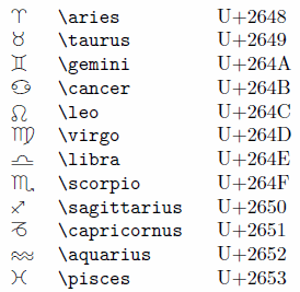
The wasysym package for LaTeX includes miscellaneous symbols, including zodiac symbols. Here are the symbols, their LaTeX commands, and their corresponding Unicode code points.

The only surprise here is that the command for Capricorn is based on the Latin form of the name: \capricornus.

Each zodiac sign is used to denote a 30° region of the sky. Since the Unicode symbols are consecutive, you can compute the code point of a symbol from the longitude angle θ in degrees:

9800 + \left\lfloor \frac{\theta}{30} \right\rfloor

Here 9800 is the decimal form of 0x2648, and the half brackets are the floor symbol, i.e. round down to the nearest integer.

Here’s the LaTeX code that produced the table.

\documentclass{article}
\usepackage{wasysym}
\begin{document}

\begin{table}
\begin{tabular}{lll}
\aries       & \verb|\aries       | & U+2648 \\
\taurus      & \verb|\taurus      | & U+2649 \\
\gemini      & \verb|\gemini      | & U+264A \\
\cancer      & \verb|\cancer      | & U+264B \\
\leo         & \verb|\leo         | & U+264C \\
\virgo       & \verb|\virgo       | & U+264D \\
\libra       & \verb|\libra       | & U+264E \\
\scorpio     & \verb|\scorpio     | & U+264F \\
\sagittarius & \verb|\sagittarius | & U+2650 \\
\capricornus & \verb|\capricornus | & U+2651 \\
\aquarius    & \verb|\aquarius    | & U+2652 \\
\pisces      & \verb|\pisces      | & U+2653 \\
\end{tabular}
\end{table}
\end{document}

By the way, you can use the Unicode values in HTML by replacing U+ with &#x and adding a semicolon on the end.

More LaTeX posts