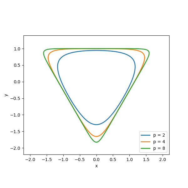
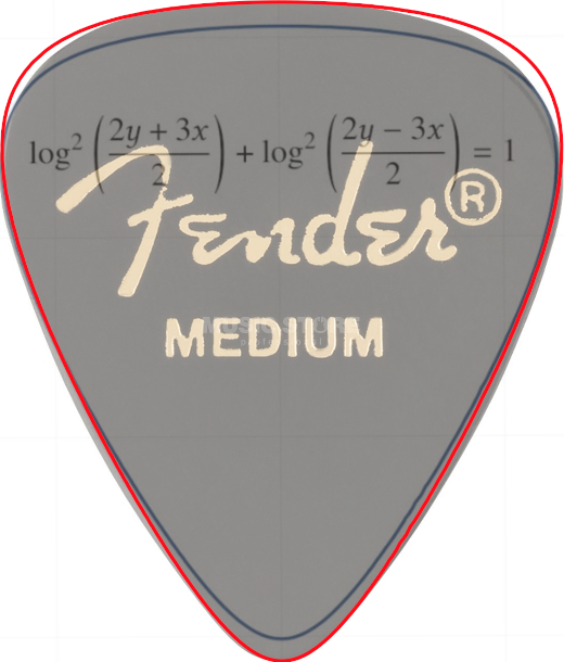
The previous post constructed a triangular analog of the squircle, the unit circle in the p-norm where p is typically around 4. The case p = 2 is a Euclidean circle and the limit as p → ∞ is a Euclidean square.
The previous post introduced three functions Li(x, y) such that the level set of each function
![]()
forms a side of a triangle. Then it introduced a soft penalty for each L being away 1, and the level sets of that penalty function formed the rounded triangles we were looking for.
Another approach would be to change the L‘s slightly so that the sides are the levels sets Li(x, y) = 0. The advantage to this formulation is that the product of three numbers is 0 if and only if one of the numbers is zero. That means if we define
![]()
then the set of points
![]()
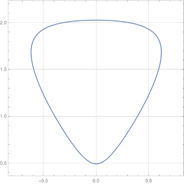
corresponds to the three lines when c = 0 and the level sets for small c > 0 are nearly triangles. The level sets will be smooth if the gradient is non-zero, i.e. c is not zero.
This approach is not unique to triangles. You could create smooth approximations any polygon by multiplying linear functions that define the sides. Or you could do something similar with curved arcs.
If we define our L’s by

then our curves will be the level sets of
![]()
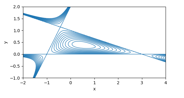
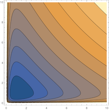
A few level sets are shown below. The level set for c = 0 is the straight lines.
Note the level sets are not connected. If you’re interested in approximate triangles, you want the components that are inside the triangle.


![\partial f(x) = \left\{ \begin{array}{cl} 1 & \text{if } x > 0 \\<br /> \left[0,1\right] & \text{if } x = 0 \\<br /> 0 & \text{if } x < 0 \end{array} \right.](https://www.johndcook.com/subgradient.svg)