I seem to run into Catalan numbers fairly regularly. This evening I ran into Catalan numbers while reading Stephen Wolfram’s book Combinators: A Centennial View [1]. Here’s the passage.

The number of combinator expressions of size n grows like

{2, 4, 16, 80, 448, 2688, 16896, 109824, 732160, 4978688}

or in general

2ⁿ CatalanNumber[n-1] = 2ⁿ Binomial[2n – 2, n – 1]/n

or asymptotically:

Specifically, Wolfram is speaking about S and K combinators. (See a brief etymology of combinator names here.)

The Catalan numbers are defined by

Replacing n with n-1 above shows that

CatalanNumber[n-1] = Binomial[2n – 2, n – 1]/n

as claimed above.

The formula for the number of combinators is easy to derive [1]. There are 2ⁿ ways to write down a string of n characters that are either S or K. Then the number of ways to add parentheses is the (n-1)st Catalan number, as explained here.

Wolfram’s asymptotic expression is closely related to a blog post I wrote two weeks ago called kn choose n. That post looked at asymptotic formulas for

and Catalan numbers correspond to f(n, 2)/(n + 1). That post showed that

The asymptotic estimate stated in Wolfram’s book follows by replacing n with n-1 above and multiplying by 2ⁿ/n. (Asymptotically there’s no difference between n and n-1 in the denominator.)

More posts on Catalan numbers

• How many ways can you parenthesize an expression?
• Calculating ζ(3) faster
• Large matrices rarely have saddle points
• Number of digits in Catalan numbers

[1] Believe it or not, I’m reading this in connection with a consulting project. When Wolfram’s book first came out, my reaction was something like “Interesting, though it’ll never be relevant to me.” Famous last words.

[2] Later in the book Wolfram considers combinators made only using S. This is even simpler since are no choices of symbols; the only choice is where to put the parentheses, and CatalanNumber[n-1] tells you how many ways that can be done.

A few days ago I wrote a brief post showing an interesting pattern that comes from plotting sin(1), sin(2), sin(3), etc.

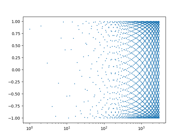
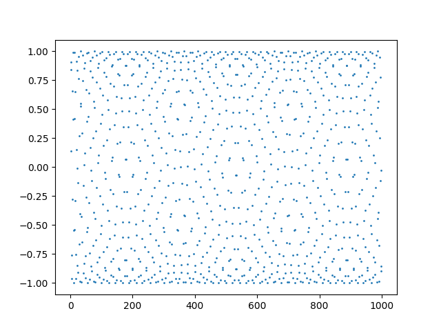
That post uses a logarithmic scale on the horizontal axis. You get a different, but also interesting, pattern when you use a linear scale.

Someone commented that this looks like a projection of a carbon nanotube, and I think they’re right.

Let’s generalize this by plotting sin(kn) for integer n. The plot above corresponds to k = 1. Tiny changes to k make a big difference in the appearance of the plot.

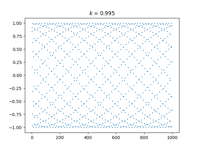
Here’s k = 0.995:

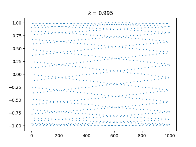
And here’s k = 1.005:

And here’s an animated plot, continuously changing k from 0.99 to 1.01.

This animation was created using the following Mathematica code.

    Animate[ListPlot[Table[Sin[k n], {n, 1, 1000}]], {k, 0.99, 1.01}, 
            AnimationRate -> 0.001, TrackedSymbols :> {k}]

The symbols ≪ and ≫ may be confusing the first time you see them, but they’re very handy.

The symbol ≪ means “much less than, and its counterpart ≫ means “much greater than”. Here’s a little table showing how to produce the symbols.

    |-------------------+---------+-------+------|
    |                   | Unicode | LaTeX | HTML |
    |-------------------+---------+-------+------|
    | Much less than    | U+226A  | \ll   | ≪ |
    | Much greater than | U+226B  | \gg   | ≫ |
    |-------------------+---------+-------+------|

Of course “much” depends on context. Is 5 much less than 7? It is if you’re describing the height of people in feet, but maybe not in the context of prices of hamburgers in dollars.

Sometimes you’ll see ≫, or more likely >> (two greater than symbols), as slang for “is much better than.” For example, someone might say “prototype >> powerpoint” to convey that a working prototype is much better than a PowerPoint pitch deck.

The symbols ≪ and ≫ can make people uncomfortable because they’re insider jargon. You have to know the context to understand how to interpret them, but they’re very handy if you are an insider. All jargon is like this.

Below are some examples of ≪ and ≫ in practice.

Square root approximation

You might see somewhere that for |b| ≪ a, the following approximation holds:

So when is |b| much less than a? That’s up to you. If, in your context, you decide that b/a is small, the approximation error will be an order of magnitude smaller.

Suppose you need to know √103 to a couple decimal places. Here a = 100 and b = 3. The ratio b/a = 0.03, and your error should be small relative to 0.03, so the approximation above should be good enough. Let’s see if that’s right.

The approximation above gives

√103 ≈ √100 + 3/2√100 = 10 + 3/20 = 10.15

and the exact value of √103 is 10.14889…, and so we did get two correct decimal places, and we nearly got three.

Sine approximation

Rather than saying a variable is “small,” we might say it is much less than 1. For example, you may see

sin θ ≈ θ

for |θ| ≪ 1. If θ is small, the error in the approximation above is very small.

A few years I wrote a 700-word blog post unpacking in detail what the previous sentence means. A lot of people memorize “You can replace sin θ with θ for small angles” without thoroughly understanding what this means. How small is small enough? The post explains how to know.

Stirling’s formula

Sometimes you see something like n ≫ 1 to indicate that n must be large. For example, Stirling’s formula for factorials says

for n ≫ 1. For instance, if n = 10, the approximation above has an error of less than 1%.

Note that the approximation error above is small relative to the exact value. The relative error is small, not the absolute error. The error in the example is more than 30,000, but this value is small relative to 10! = 3,628,800.

Asymmetry between small and large

It’s often harder to tell from context when something is large than when it is small.

If an approximation holds for |x| ≪ 1, there’s often an implicit power series in the background, and the error is on the order of x². That’s the case in our square root approximation above. The sine approximation is even better, with error on the order of x³.

But if an approximation holds for x ≫ 1, there’s often an implicit asymptotic series in the background, and these are more subtle. You likely need more context to how large x needs to be for a particular application.

Related posts

• Unicode <-> LaTeX
• It doesn’t matter much if the tape measure is straight
• Applied math