Avoiding underflow in Bayesian computations

Posted on 26 July 2012 by John

Here’s a common problem that arises in Bayesian computation. Everything works just fine until you have more data than you’ve seen before. Then suddenly you start getting infinite, NaN, or otherwise strange results. This post explains what might be wrong and how to fix it.

A posterior density is (proportional to) a likelihood function times a prior distribution. The likelihood function is a product. The number of data points is the number of terms in the product. If these numbers are less than 1, and you multiply enough of them together, the result will be too small to represent in a floating point number and your calculation will underflow to zero. Then subsequent operations with this number, such as dividing it by another number that has also underflowed to zero, may produce an infinite or NaN result.

The instinctive reaction regarding underflow or overflow is to use logs. And often that works. If you wanted to know where the maximum of the posterior density occurs, you could find the maximum of the logarithm of the posterior density. But in Bayesian computations you often need to integrate the posterior density times some functions. Now you cannot just work with logs because logs and integrals don’t commute.

One way around the problem is to multiply the integrand by a constant so large that there is no danger of underflow. Multiplying by constants does commute with integration.

So suppose your integrand is on the order of 10^−400, far below the smallest representable number. Do you need extended precision arithmetic? No, you just need to understand your problem.

If you multiply your integrand by 10^400 before integrating, then your integrand is roughly 1 in magnitude. Then do you integration, and remember that the result is 10^400 times the actual value.

You could take the following steps.

Find m, the maximum of the log of the integrand.
Let I be the integral of exp( log of the integrand − m ).
Keep track that your actual integral is exp(m) I, or that its log is m + log I.

Note that you can be extremely sloppy in this process. You don’t need an accurate estimate of the maximum of the integrand per se. If you’re within a few dozen orders of magnitude, for example, that could be sufficient to carry out your integration without underflow.

One way to estimate the maximum is to use a frequentist estimator of your parameters as an approximate MLE, and assume that this is approximately where your posterior density takes on its maximum value. This might actually be very accurate, but it doesn’t need to be.

Note also that it’s OK if some of the evaluations of your integrand underflow to zero. You just don’t want the entire integral to underflow to zero. Places where the integrand is many orders of magnitude less than its maximum don’t contribute to the integration anyway. (It’s important that your integration pays attention to the region where the integrand is largest. A naive integration could entirely miss the most important region and completely underestimate the integral. But that’s a matter for another blog post.)

Monkeying with Bayes’ theorem

Posted on 9 March 2012 by John

In Peter Norvig’s talk The Unreasonable Effectiveness of Data, starting at 37:42, he describes a translation algorithm based on Bayes’ theorem. Pick the English word that has the highest posterior probability as the translation. No surprise here. Then at 38:16 he says something curious.

So this is all nice and theoretical and pure, but as well as being mathematically inclined, we are also realists. So we experimented some, and we found out that when you raise that first factor [in Bayes’ theorem] to the 1.5 power, you get a better result.

In other words, if we change Bayes’ theorem (!) the algorithm works better. He goes on to explain

Now should we dig up Bayes and notify him that he was wrong? No, I don’t think that’s it. …

I imagine most statisticians would respond that this cannot possibly be right. While it appears to work, there must be some underlying reason why and we should find that reason before using an algorithm based on an ad hoc tweak.

While such a reaction is understandable, it’s also a little hypocritical. Statisticians are constantly drawing inference from empirical data without understanding the underlying mechanisms that generate the data. When analyzing someone else’s data, a statistician will say that of course we’d rather understand the underlying mechanism than fit statistical models, that’s just not always possible. Reality is too complicated and we’ve got to do the best we can.

I agree, but that same reasoning applied at a higher level of abstraction could be used to accept Norvig’s translation algorithm. Here’s this model (derived from spurious math, but we’ll ignore that). Let’s see empirically how well it works.

The universal solvent of statistics

Posted on 1 February 2012 by John

Andrew Gelman just posted an interesting article on the philosophy of Bayesian statistics. Here’s my favorite passage.

This reminds me of a standard question that Don Rubin … asks in virtually any situation: “What would you do if you had all the data?” For me, that “what would you do” question is one of the universal solvents of statistics.

Emphasis added.

I had not heard Don Rubin’s question before, but I think I’ll be asking it often. It reminds me of Alice’s famous dialog with the Cheshire Cat:

“Would you tell me, please, which way I ought to go from here?”

“That depends a good deal on where you want to get to,” said the Cat.

“I don’t much care where–” said Alice.

“Then it doesn’t matter which way you go,” said the Cat.

Cheshire Cat

Related post: Irrelevant uncertainty

Six analysis and probability diagrams

Posted on 17 January 2012 by John

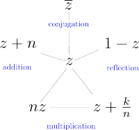
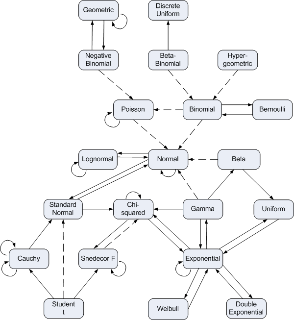
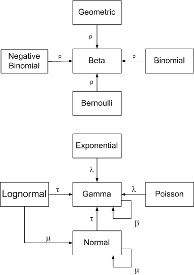
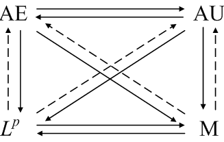
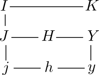
Here are a few diagrams I’ve created that summarize relationships in analysis and probability. Click on a thumbnail image to go to a page with the full image and explanatory text.

Special functions

Gamma and related functions

Probability distributions

Conjugate priors

Convergence theorems

Bessel functions

Interpreting statistics

Posted on 13 January 2012 by John

From Matt Briggs:

I challenge you to find me in any published statistical analysis, outside of an introductory textbook, a confidence interval given the correct interpretation. If you can find even one instance where the [frequentist] confidence interval is not interpreted as a [Bayesian] credible interval, then I will eat your hat.

Most statistical analysis is carried out by people who do not interpret their results correctly. They carry out frequentist procedures and then give the results a Bayesian interpretation. This is not simply a violation of an academic taboo. It means that people generally underestimate the uncertainty in their conclusions.

Bad logic, but good statistics

Posted on 28 November 2011 by John

Ad hominem arguments are bad logic, but good (Bayesian) statistics. A statement isn’t necessarily false because it comes from an unreliable source, though it is more likely to be false.

Some people are much more likely to know what they’re talking about than others, depending on context. You’re more likely to get good medical advice from a doctor than from an accountant, though the former may be wrong and the latter may be right. (Actors are not likely to know what they’re talking about when giving advice regarding anything but acting, though that doesn’t stop them.)

Ad hominem guesses are a reasonable way to construct a prior, but the prior needs to be updated with data. Given no other data, the doctor is more likely to know medicine than the accountant is. Assuming a priori that both are equally likely to be correct may be “fair,” but it’s not reasonable. However, as you gather data on the accuracy of each, you could change your mind. The posterior distribution could persuade you that you’ve been talking to a quack doctor or an accountant who is unusually knowledgeable of medicine.

Related post: Musicians, drunks, and Oliver Cromwell

Leading digits of factorials

Posted on 19 October 2011 by John

Suppose you take factorials of a lot of numbers and look at the leading digit of each result. You could argue that there’s no apparent reason that any digit would be more common than any other, so you’d expect each of the digits 1 through 9 would come up 1/9 of the time. Sounds plausible, but it’s wrong.

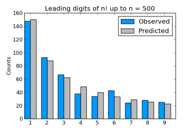
The leading digits of factorials follow Benford’s law as described in the previous post. In fact, factorials follow Benford’s law even better than physical constants do. Here’s a graph of the leading digits of the factorials of 1 through 500.

In the remainder of this post, I’ll explain why Benford’s law should apply to factorials, make an aside on statistics, and point out an interesting feature of the Python code used to generate the chart above.

Why Benford’s law applies

Here’s a hand-waving explanation. One way to justify Benford’s law is to say that physical constants are uniformly distributed, but on a logarithmic scale. The same is true for factorials, and it’s easier to see why.

The leading digits of the logarithms depend on their logarithms in base 10. The gamma function extends the factorial function and it is log-convex. The logarithm of the gamma function is fairly flat (see plot here), and so the leading digits of the log-gamma function applied to integers are uniformly distributed on a logarithmic scale. (I’ve mixed logs base 10 and natural logs here, but that doesn’t matter. All logarithms are the same up to a multiplicative constant. So if a plot is nearly linear on a log10 scale, it’s nearly linear on a natural log scale.)

Update: Graham gives a link in the comments below to a paper proving that factorials satisfy Benford’s law exactly in the limit.

Uniform on what scale?

This example brings up an important principle in statistics. Some say that if you don’t have a reason to assume anything else, use a uniform distribution. For example, some say that a uniform prior is the ideal uninformative prior for Bayesian statistics. But you have to ask “Uniform on what scale?” It turns out that the leading digits of physical constants and factorials are indeed uniformly distributed, but on a logarithmic scale.

Python integers and floating point

I used nearly the same code to produce the chart above as I used in its counterpart in the previous post. However, one thing had to change: I couldn’t compute the leading digits of the factorials the same way. Python has extended precision integers, so I can compute 500! factorial without overflowing. Using floating point numbers, I could only go up to 170!. But when I used my previous code to find the leading digit, it first tried to apply log10 to an integer larger than the largest representable floating point number and failed. Converting numbers such as 500! to floating point numbers will overflow. (See Floating point numbers are a leaky abstraction.)

The solution was to find the leading digit using only integer operations.

    def leading_digit_int(n):
        while n > 9:
            n = n/10
        return n

This code works fine for numbers like 500! or even larger.

A Bayesian view of Amazon Resellers

Posted on 27 September 2011 by John

I was buying a used book through Amazon this evening. Three resellers offered the book at essentially the same price. Here were their ratings:

94% positive out of 85,193 reviews
98% positive out of 20,785 reviews
99% positive out of 840 reviews

Which reseller is likely to give the best service? Before you assume it’s the seller with the highest percentage of positive reviews, consider the following simpler scenario.

Suppose one reseller has 90 positive reviews out of 100. The other reseller has two reviews, both positive. You could say one has 90% approval and the other has 100% approval, so the one with 100% approval is better. But this doesn’t take into consideration that there’s much more data on one than the other. You can have some confidence that 90% of the first reseller’s customers are satisfied. You don’t really know about the other because you have only two data points.

A Bayesian view of the problem naturally incorporates the amount of data as well as its average. Let θ_A be the probability of a customer being satisfied with company A‘s service. Let θ_B be the corresponding probability for company B. Suppose before we see any reviews we think all ratings are equally likely. That is, we start with a uniform prior distribution θ_A and θ_B. A uniform distribution is the same as a beta(1, 1) distribution.

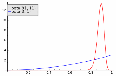
After observing 90 positive reviews and 10 negative reviews, our posterior estimate on θ_A has a beta(91, 11) distribution. After observing 2 positive reviews, our posterior estimate on θ_B has a beta(3, 1) distribution. The probability that a sample from θ_A is bigger than a sample from θ_B is 0.713. That is, there’s a good chance you’d get better service from the reseller with the lower average approval rating.

beta(91,11) versus beta(3,1)

Now back to our original question. Which of the three resellers is most likely to satisfy a customer?

Assume a uniform prior on θ_X, θ_Y, and θ_Z, the probabilities of good service for each reseller. The posterior distributions on these variables have distributions beta(80082, 5113), beta(20370, 417), and beta(833, 9).

These beta distributions have such large parameters that we can approximate them by normal distributions with the same mean and variance. (A beta(a, b) random variable has mean a/(a+b) and variance ab/((a+b)²(a+b+1)).) The variable with the most variance, θ_Z, has standard deviation 0.003. The other variables have even smaller standard deviation. So the three distributions are highly concentrated at their mean values with practically non-overlapping support. And so a sample from θ_X or θ_Y is unlikely to be higher than a sample from θ_Z.

In general, going by averages alone works when you have a lot of customer reviews. But when you have a small number of reviews, going by averages alone could be misleading.

Thanks to Charles McCreary for suggesting the xkcd comic.

Big data and humility

Posted on 22 September 2011 by John

One of the challenges with big data is to properly estimate your uncertainty. Often “big data” means a huge amount of data that isn’t exactly what you want.

As an example, suppose you have data on how a drug acts in monkeys and you want to infer how the drug acts in humans. There are two sources of uncertainty:

How well do we really know the effects in monkeys?
How well do these results translate to humans?

The former can be quantified, and so we focus on that, but the latter may be more important. There’s a strong temptation to believe that big data regarding one situation tells us more than it does about an analogous situation.

I’ve seen people reason as follows. We don’t really know how results translate from monkeys to humans (or from one chemical to a related chemical, from one market to an analogous market, etc.). We have a moderate amount of data on monkeys and we’ll decimate it and use that as if it were human data, say in order to come up with a prior distribution.

Down-weighting by a fixed ratio, such as 10 to 1, is misleading. If you had 10x as much data on monkeys, would you as much about effects in humans as if the original smaller data set were collected on people? What if you suddenly had “big data” involving every monkey on the planet. More data on monkeys drives down your uncertainty about monkeys, but does nothing to lower your uncertainty regarding how monkey results translate to humans.

At some point, more data about analogous cases reaches diminishing return and you can’t go further without data about what you really want to know. Collecting more and more data about how a drug works in adults won’t help you learn how it works in children. At some point, you need to treat children. Terabytes of analogous data may not be as valuable as kilobytes of highly relevant data.

Bayes isn’t magic

Posted on 6 September 2011 by John

If a study is completely infeasible using traditional statistical methods, Bayesian methods are probably not going to rescue it. Bayesian methods can’t squeeze blood out of a turnip.

The Bayesian approach to statistics has real advantages, but sometimes these advantages are oversold. Bayesian statistics is still statistics, not magic.

Bayesian