Sine series for a sine

Posted on 7 April 2020 by John

The Fourier series of an odd function only has sine terms—all the cosine coefficients are zero—and so the Fourier series is a sine series.

What is the sine series for a sine function? If the frequency is an integer, then the sine series is just the function itself. For example, the sine series for sin(5x) is just sin(5x). But what if the frequency is not an integer?

For an odd function f on [-π, π] we have

$f(x) = \sum_{n=0}^\infty c_n \sin(n x)$

where the coefficients are given by

$c_n = \frac{1}{\pi} \int_{-\pi}^\pi f(x) \sin(nx)\, dx$

So if λ is not an integer, the sine series coefficients for sin(λx) are given by

$c_n = 2\sin(\lambda \pi) (-1)^n \,\frac{ n}{\pi(\lambda^2 - n^2)}$

The series converges slowly since the coefficients are O(1/n).

For example, here are the first 15 coefficients for the sine series for sin(1.6x).

And here is the corresponding plot for sin(2.9x).

As you might expect, the coefficient of sin(3x) is nearly 1, because 2.9 is nearly 3. What you might not expect is that the remaining coefficients are fairly large.

Update: After writing this post I wrote another on the rate of convergence for Fourier series. In general, the smoother the function, the faster the Fourier series converges and vice versa, with some fine print.

The sine function above is perfectly smooth, but it’s Fourier series converges slowly. How can that be? The Fourier series is defined for periodic functions. If k is not an integer and we force sin(kx) to be a function with period 2π, it is not continuous. When we extend sin(kx) to make it periodic, there’s a jump discontinuity at the ends of each period.

Look back at

$f(x) = \sum_{n=0}^\infty c_n \sin(n x)$

This equation can’t hold everywhere. If k is not an integer and f(x) = sin(kx), then the right size is zero at π but the left is not. In fact we’ll see Gibbs phenomenon at π because of the discontinuity there.

Exponential sum for the new year

Posted on 1 January 2018 by John

Exponential sums can make intricate patterns. Last year I made a page that displays a different page each day, using the month, day, and year as parameters in the expression below. The images plot the partial sums of this sum.

$\sum_{n=0}^N \exp\left( 2\pi i \left( \frac{n}{m} + \frac{n^2}{d} + \frac{n^3}{y} \right ) \right )$

This was yesterday’s image.

Image of the day, New Year's Eve.

Today’s image is surprisingly plain if we use y = 18.

This is in part because the least common multiple of 1, 1, and 18 is 18. The image could have no more than 18 vertices. In fact, it has only 6 vertices because the summand above has period 6.

But if we use y = 2018 we get something much more complex.

The Exponential Sum of the Day page will use y = 18 this year. There will be a few simple images this year but there will also be lots of surprises.

Moment generating functions and connections to other things

Posted on 5 December 2017 by John

This post relates moment generating functions to the Laplace transform and to exponential generating functions. It also brings in connections to the z-transform and the Fourier transform.

Thanks to Brian Borchers who suggested the subject of this post in a comment on a previous post on transforms and convolutions.

Moment generating functions

The moment generating function (MGF) of a random variable X is defined as the expected value of exp(tX). By the so-called rule of the unconscious statistician we have

$M_X(t) \equiv \mathrm{E}[e^{tX}] = \int_{-\infty}^\infty e^{tx} f_X(x)\, dx$

where f_X is the probability density function of the random variable X. The function M_X is called the moment generating function of X because it’s nth derivative, evaluated at 0, gives the nth moment of X, i.e. the expected value of Xⁿ.

Laplace transforms

If we flip the sign on t in the integral above, we have the two-sided Laplace transform of f_X. That is, the moment generating function of X at t is the two-sided Laplace transform of f_X at –t. If the density function is zero for negative values, then the two-sided Laplace transform reduces to the more common (one-sided) Laplace transform.

Exponential generating functions

Since the derivatives of M_X at zero are the moments of X, the power series for M_X is the exponential generating function for the moments. We have

$M_X(t) = m_0 + m_1t + \frac{m_2}{2}t^2 + \frac{m_3}{3!} t^3 + \cdots$

where m_n is the nth moment of X.

Other generating functions

This terminology needs a little explanation since we’re using “generating function” two or three different ways. The “moment generating function” is the function defined above and only appears in probability. In combinatorics, the (ordinary) generating function of a sequence is the power series whose coefficient of xⁿ is the nth term of the sequence. The exponential generating function is similar, except that each term is divided by n!. This is called the exponential generating series because it looks like the power series for the exponential function. Indeed, the exponential function is the exponential generating function for the sequence of all 1’s.

The equation above shows that M_X is the exponential generating function for m_n and the ordinary generating function for m_n/n!.

If a random variable Y is defined on the integers, then the (ordinary) generating function for the sequence Prob(Y = n) is called, naturally enough, the probability generating function for Y.

The z-transform of a sequence, common in electrical engineering, is the (ordinary) generating function of the sequence, but with x replaced with 1/z.

Characteristic functions

The characteristic function of a random variable is a variation on the moment generating function. Rather than use the expected value of tX, it uses the expected value of itX. This means the characteristic function of a random variable is the Fourier transform of its density function.

Characteristic functions are easier to work with than moment generating functions. We haven’t talked about when moment generating functions exist, but it’s clear from the integral above that the right tail of the density has to go to zero faster than e^–x, which isn’t the case for fat-tailed distributions. That’s not a problem for the characteristic function because the Fourier transform exists for any density function. This is another example of how complex variables simplify problems.

Shannon wavelet

Posted on 4 December 2017 by John

The Shannon wavelet has an interesting plot:

Shannon wavelet

Given the complexity of the plot, the function definition is surprisingly simple:

$\frac{1}{\pi t} (\sin 2\pi t - \sin\pi t)$

The Fourier transform is even simpler: it’s the indicator function of [-2π, -π] ∪ [π, 2π], i.e. the function that is 1 on the intervals [-2π, -π] and [π, 2π] but zero everywhere else.

The Shannon wavelet is orthogonal to integer translates of itself. This isn’t obvious in the time domain, but it’s easy to prove in the frequency domain using Parseval’s theorem.

Here’s a plot of the original wavelet and the wavelet shifted to the left by 3:

Two Shannon wavelets

And here’s a plot of the product of the two wavelets. It’s plausible that the areas above and below the x-axis cancel out each other, and indeed they do.

Product of two Shannon wavelets

Related post: Sinc and Jinc integrals

Fourier-Bessel series and Gibbs phenomena

Posted on 4 November 2017 by John

Fourier-Bessel series are analogous to Fourier series. And like Fourier series, they converge pointwise near a discontinuity with the same kind of overshoot and undershoot known as the Gibbs phenomenon.

Fourier-Bessel series

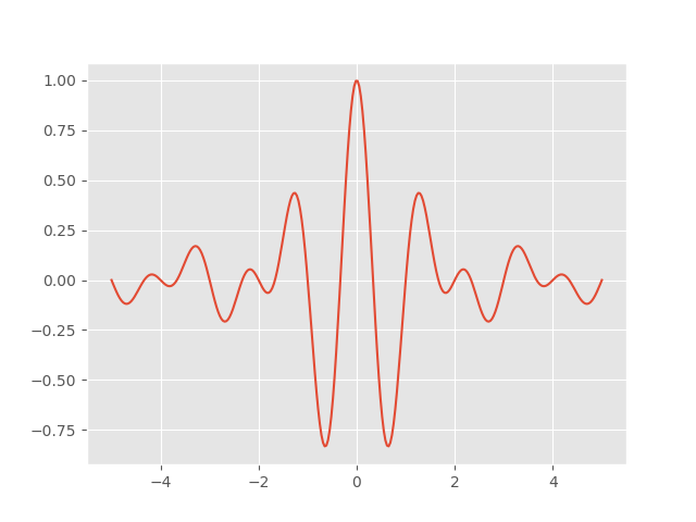
Bessel functions come up naturally when working in polar coordinates, just as sines and cosines come up naturally when working in rectangular coordinates. You can think of Bessel functions as a sort of variation on sine waves. Or even more accurately, a variation on sinc functions, where sinc(z) = sin(z)/z. [1]

A Fourier series represents a function as a sum of sines and cosines of different frequencies. To make things a little simpler here, I’ll only consider Fourier sine series so I don’t have to repeatedly say “and cosine.”

$f(z) = \sum_{n=1}^\infty c_n \sin(n \pi z)$

A Fourier-Bessel function does something similar. It represents a function as a sum of rescaled versions of a particular Bessel function. We’ll use the Bessel J₀ here, but you could pick some other J_ν.

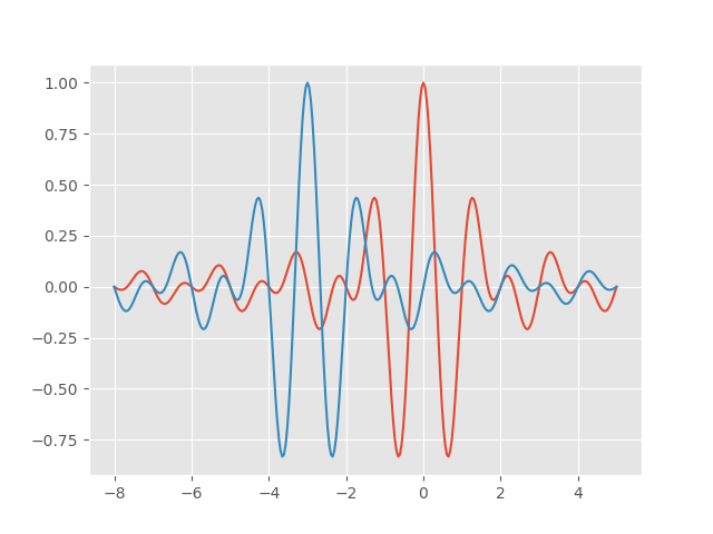
Fourier series scale the sine and cosine functions by π times integers, i.e. sin(πz), sin(2πz), sin(3πz), etc. Fourier-Bessel series scale by the zeros of the Bessel function: J₀(λ₁z), J₀(λ₂z), J₀(λ₃z), etc. where λ_n are the zeros of J₀. This is analogous to scaling sin(πz) by its roots: π, 2π, 3π, etc. So a Fourier-Bessel series for a function f looks like

$f(z) = \sum_{n=1}^\infty c_n J_0(\lambda_n z).$

The coefficients c_n for Fourier-Bessel series can be computed analogously to Fourier coefficients, but with a couple minor complications. First, the basis functions of a Fourier series are orthogonal over [0, 1] without any explicit weight, i.e. with weight 1. And second, the inner product of a basis function doesn’t depend on the frequency. In detail,

$\int_0^1 \sin(m \pi z) \, \sin(n \pi z) \, dz = \frac{\delta_{mn}}{2}.$

Here δ_mn equals 1 if m = n and 0 otherwise.

Fourier-Bessel basis functions are orthogonal with a weight z, and the inner product of a basis function with itself depends on the frequency. In detail

$\int_0^1 J_0(\lambda_m z) \, J_0(\lambda_n z) \, z\, dz = \frac{\delta_{mn}}{2} J_1(\lambda_n).$

So whereas the coefficients for a Fourier sine series are given by

$c_n = 2 \int_0^1 f(z)\, \sin(n\pi z) \,dz$

the coefficients for a Fourier-Bessel series are given by

$c_n = \frac{ 2\int_0^1 f(z)\, J_0(\lambda_n z) \, dz}{ J_1(\lambda_n)^2 }.$

Gibbs phenomenon

Fourier and Fourier-Bessel series are examples of orthogonal series, and so by construction they converge in the norm given by their associated inner product. That means that if S_N is the Nth partial sum of a Fourier series

$\lim_{N\to\infty} \int_0^1 \left( f(x) - S_N(x) \right)^2 \, dz = 0$
and the analogous statement for a Fourier-Bessel series is

$\lim_{N\to\infty} \int_0^1 \left( f(x) - S_N(x) \right)^2 \, z\, dz = 0.$

In short, the series converge in a (weighted) L² norm. But how do the series converge pointwise? A lot of harmonic analysis is devoted to answering this question, what conditions on the function f guarantee what kind of behavior of the partial sums of the series expansion.

If we look at the Fourier series for a step function, the partial sums converge pointwise everywhere except at the step discontinuity. But the way they converge is interesting. You get a sort of “bat ear” phenomena where the partial sums overshoot the step function at the discontinuity. This is called the Gibbs phenomenon after Josiah Willard Gibbs who observed the effect in 1899. (Henry Wilbraham observed the same thing earlier, but Gibbs didn’t know that.)

The Gibbs phenomena is well known for Fourier series. It’s not as well known that the same phenomenon occurs for other orthogonal series, such as Fourier-Bessel series. I’ll give an example of Gibbs phenomenon for Fourier-Bessel series taken from [2] and give Python code to visualize it.

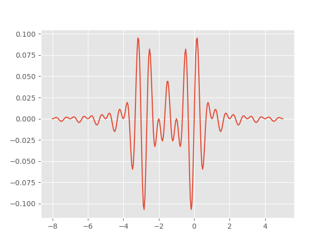
We take our function f(z) to be 1 on [0, 1/2] and 0 on (1/2, 1]. It works out that

$c_n = \frac{1}{\lambda_n} \frac{J_1(\lambda_n / 2)}{ J_1(\lambda_n)^2 }.$

Python code and plot

Here’s the plot with 100 terms. Notice how the partial sums overshoot the mark to the left of 1/2 and undershoot to the right of 1/2.

Plot showing Gibbs phenomena for Fourier-Bessel series

Here’s the same plot with 1,000 terms.

Gibbs phenomena for 1000 terms of Fourier-Bessel series

Here’s the Python code that produced the plot.

    import matplotlib.pyplot as plt
    from scipy.special import j0, j1, jn_zeros
    from scipy import linspace

    N = 100 # number of terms in series

    roots = jn_zeros(0, N)
    coeff = [j1(r/2) / (r*j1(r)**2) for r in roots]
    z = linspace(0, 1, 200)

    def partial_sum(z):
        return sum( coeff[i]*j0(roots[i]*z) for i in range(N) )

    plt.plot(z, partial_sum(z))
    plt.xlabel("z")
    plt.ylabel("{}th partial sum".format(N))
    plt.show()

Footnotes

[1] To be precise, as z goes to infinity

$J_nu(z) sim sqrt{frac{2}{pi z}} cosleft(z - frac{1}{2} nu pi - frac{pi}{4} right)$

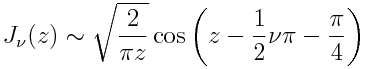
and so the Bessel functions are asymptotically proportional to sin(z – φ)/√z for some phase shift φ.

[2] The Gibbs’ phenomenon for Fourier-Bessel Series. Temple H. Fay and P. Kendrik Kloppers. International Journal of Mathematical Education in Science and Technology. 2003. vol. 323, no. 2, 199-217.

Animated exponential sum

Posted on 4 November 2017 by John

I’m experimenting with making animated versions of the kinds of images I wrote about in my previous post. Here’s an animated version of the exponential sum of the day for 12/4/17.

Why that date? I wanted to start with something with a fairly small period, and that one looked interesting. I’ll have to do something different for the images that have a much longer period.

Update: Now all the images on the exponential sum site have the option of showing animation. Here’s an interesting example.

Exponential sum of the day

Posted on 9 October 2017 by John

I’ve written a page that will show a different exponential sum each day, images along the line of the post Exponential sums make pretty pictures.

Here’s the page: https://www.johndcook.com/expsum/

Here are a few sample images. Small changes in the coefficients can make a big change in the appearance of the graphs.

Exponential sums make pretty pictures

Posted on 7 October 2017 by John

Exponential sums are a specialized area of math that studies series with terms that are complex exponentials. Estimating such sums is delicate work. General estimation techniques are ham-fisted compared to what is possible with techniques specialized for these particular sums. Exponential sums are closely related to Fourier analysis and number theory.

Exponential sums also make pretty pictures. If you make a scatter plot of the sequence of partial sums you can get surprising shapes. This is related to the trickiness of estimating such sums: the partial sums don’t simply monotonically converge to a limit.

The exponential sum page at UNSW [link went away] suggests playing around with polynomials with dates in the denominator. If we take that suggestion with today’s date, we get the curve below:

f(n) = n/10 + n**2/7 + n**3/17

These are the partial sums of exp(2πi f(n)) where f(n) = n/10 + n²/7 + n³/17.

[Update: You can get an image each day for the current day’s date here.]

Here’s the code that produced the image.

    import matplotlib.pyplot as plt
    from numpy import array, pi, exp, log

    N = 12000
    def f(n):
        return n/10 + n**2/7 + n**3/17 

    z = array( [exp( 2*pi*1j*f(n) ) for n in range(3, N+3)] )
    z = z.cumsum()

    plt.plot(z.real, z.imag, color='#333399')
    plt.axes().set_aspect(1)
    plt.show()

If we use logarithms, we get interesting spirals. Here f(n) = log(n)^4.1.

f(n) = log(n)**4.1

And we can mix polynomials with logarithms. Here f(n) = log(n) + n²/100.

f(n) = log(n) + n**2/100

In this last image, I reduced the number of points from 12,000 to 1200. With a large number of points the spiral nature dominates and you don’t see the swirls along the spiral as clearly.

Defining the Fourier transform on LCA groups

Posted on 27 August 2017 by John

My previous post said that all the familiar variations on Fourier transforms—Fourier series analysis and synthesis, Fourier transforms on the real line, discrete Fourier transforms, etc.—can be unified into a single theory. They’re all instances of a Fourier transform on a locally compact Abelian (LCA) group. The difference between them is the underlying group.

Given an LCA group G, the Fourier transform takes a function on G and returns a function on the dual group of G. We said this much last time, but we didn’t define the dual group; we just stated examples. We also didn’t say just how you define a Fourier transform in this general setting.

Characters and dual groups

Before we can define a dual group, we have to define group homomorphisms. A homomorphism between two groups G and H is a function h between the groups that preserves the group structure. Suppose the group operation is denoted by addition on G and by multiplication on H (as it will be in our application), saying h preserves the group structure means

h(x + y) = h(x) h(y)

for all x and y in G.

Next, let T be the unit circle, i.e. complex numbers with absolute value 1. T is a group with respect to multiplication. (Why T for circle? This is a common notation, anticipating generalization to toruses in all dimensions. A circle is a one-dimensional torus.)

Now a character on G is a continuous homomorphism from G to T. The set of all characters on G is the dual group of G. Call this group Γ. If G is an LCA group, then so is Γ.

Integration

The classical Fourier transform is defined by an integral. To define the Fourier transform on a group we have to have a way to do integration on that group. And there’s a theorem that says we can always do that. For every LCA group, there exists a Haar measure μ, and this measure is nice enough to develop our theory. This measure is essentially unique: Any two Haar measures on the same LCA group must be proportional to each other. In other words, the measure is unique up to multiplying by a constant.

On a discrete group—for our purposes, think of the integers and the integers mod m—Haar measure is just counting; the measure of a set is the number of things in the set. And integration with respect to this measure is summation.

Fourier transform defined

Let f be a function in L¹(G), i.e. an absolutely integrable function on G. Then the Fourier transform of f is a function on Γ defined by

$\hat{f}(\gamma) = \int_G f(x)\, \gamma(-x) \, d\mu$

What does this have to do with the classical Fourier transform? The classical Fourier transform takes a function of time and returns a function of frequency. The correspondence between the classical Fourier transform and the abstract Fourier transform is to associate the frequency ω with the character that takes x to the value exp(iωx).

There are multiple slightly different conventions for the classical Fourier transform cataloged here. These correspond to different constant multiples in the choice of measure on G and Γ, i.e. whether to divide by or multiply by √(2π), and in the correspondence between frequencies and characters, whether ω corresponds to exp(±iωx) or exp(±2πiωx).

Unified theory of Fourier transforms

Posted on 26 August 2017 by John

You can take a periodic function and analyze it into its Fourier coefficients, or use the Fourier coefficients in a sum to synthesize a periodic function. You can take the Fourier transform of a function defined on the whole real line and get another such function. And you can compute the discrete Fourier transform via the FFT algorithm.

Is there a general theory that unifies all these related but different things? Why yes, yes there is.

Groups

Everything in the opening paragraph is simply a Fourier transform, each in a different context. And the contexts correspond to groups. Specifically, locally compact Abelian groups.

Some of these groups are easier to see than others. Clearly the real numbers with addition form a group: the sum of two real numbers is a real number, etc. But where are the groups in the other contexts?

You can think of a periodic function as a function on a circle; the function values have to agree at both ends of an interval, so you might as well think of those two points as the same point, i.e. join them to make a circle. Shifting along an interval, wrapping around if necessary, corresponds to a rotation of the circle, and rotations form a group. So analyzing a periodic function in to a set of Fourier coefficients is a Fourier transform on the circle.

You can think of a set of Fourier coefficients as a function on the integers, mapping n to the nth coefficient. Synthesizing a set of Fourier coefficients into a periodic function is a Fourier transform on the group of integers.

What about a discrete Fourier transform (DFT)? If you have a function sampled at m points, you could think of those points as the group of integers mod m. Your sampled points constitute a function on the integers mod m, and the DFT is a Fourier transform on that group.

Note that the DFT is a Fourier transform in its own right. It’s not an approximation per se, though it’s nearly always used as part of an approximation process. You can start with a continuous function, approximate it by a finite set of samples, compute the DFT of these samples, and the result will give you an approximation to the Fourier transform of the original continuous function.

What about functions of several variables? These are functions on groups too. A function of two real variables, for example, is a function on R², which is a group with (vector) addition.

Dual groups

A Fourier transform takes a function defined on a group and returns a function defined on the dual of that group. I go into exactly what a dual group is in my next post, but for now, just note that the Fourier transform takes a function defined on one group and returns a function defined on another group.

The dual of the circle is the integers, and vice versa. That’s why the Fourier transform of a function on the circle is an infinite set of Fourier coefficients, which we think of as a function on the integers. The Fourier transform of the function on the integers, i.e. a set of Fourier coefficients, is a function on the circle, i.e. a periodic function.

The dual group of the real numbers is the real numbers again. That’s why the Fourier transform of a function on the real line is another function on the real line.

The integers mod m is also its own dual group. So the DFT takes a set of m numbers and returns a set of m numbers.

Locally compact Abelian (LCA) groups

What do locally compact and Abelian mean? And why do we make these assumptions?

Let’s start with Abelian. This just means that the group operation is commutative. When we’re adding real numbers, or composing rotations of a circle, these operations are commutative.

Locally compactness is a more technical requirement. The circle is compact, and so are the integers mod m. But if we restricted out attention to compact groups, that would leave out the integers and the real numbers. These spaces are not compact, but they’re locally compact, and that’s enough for the theory to go through.

It turns out that LCA groups are a sort of theoretical sweet spot. Assuming groups are LCA is general enough to include the examples we care about the most, but it’s not so general that the theory becomes harder and the results less powerful.

More connections

This post relates Fourier series (analysis and synthesis) to Fourier transforms (on the real line) by saying they’re both special cases of Fourier analysis on LCA groups. There are a couple other ways to connect Fourier series and Fourier transforms.

You can take the Fourier transform (not Fourier series) of a periodic function two ways: by restricting it to one period and defining it to be zero everywhere else, or by letting it repeat forever across the real line and taking the Fourier transform in the sense of generalized functions. You can read more about these two approaches in this post.

More posts on Fourier series