A parabola, a triangle, and a circle

Posted on 18 June 2023 by John

Let P be a parabola. Draw tangents to P at three different points. These three lines intersect to form a triangle.

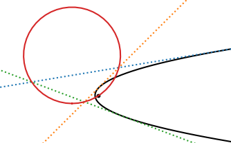
Theorem: The circumcircle of this triangle passes through the focus of P. [1]

In the image above, the dashed lines are tangents and the black dot is the focus of the parabola.

(See this post for an explanation of what focus and directrix mean.)

By the way, creating the image above required finding the circle through the three intersection points. See the previous post for how to find such a circle.

[1] Ross Honsberger. Episodes in Nineteenth and Twentieth Century Euclidean Geometry. Mathematical Association of America. 1995. Page 47.

Equation of a circle through three points

Posted on 18 June 2023 by John

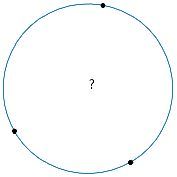
Three given points on a circle with unknown center

A few months ago I wrote about several equations that come up in geometric calculations that all have the form of a determinant equal to 0, where one column of the determinant is all 1s.

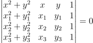
The equation of a circle through three points (x₁, y₁), (x₂, y₂), and (x₃, y₃) has this form:

$\begin{vmatrix} x^2 + y^2 & x & y & 1 \\ x_1^2 + y_1^2 & x_1 & y_1 & 1 \\ x_2^2 + y_2^2 & x_2 & y_2 & 1 \\ x_3^2 + y_3^2 & x_3 & y_3 & 1 \\ \end{vmatrix} = 0$

This is elegant equation, but it’s not in a form that’s ready to program. This post will start with the equation above and conclude with code.

Let M_ij be the determinant of the minor of the (i, j) element of the matrix above. That is, M_ij is the determinant of the 3 × 3 matrix obtained by deleting the ith row and jth column. Then we can expand the determinant above by minors of the last column to get

$M_{11}(x^2 + y^2) - M_{12}x + M_{13}y - M_{14} = 0$

which we can rewrite as

$x^2 + y^2 -\frac{M_{12}}{M_{11}} x + \frac{M_{13}}{M_{11}} y - \frac{M_{14}}{M_{11}} = 0.$

A circle with center (x₀, y₀) and radius r₀ has equation

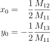
By equating the coefficients x and y in the two previous equations we have

$\begin{align*} x_0 &= \phantom{-}\frac{1}{2} \frac{M_{12}}{M_{11}} \\ y_0 &= -\frac{1}{2} \frac{M_{13}}{M_{11}} \\ \end{align*}$

Next we expand the determinant minors in more explicit form.

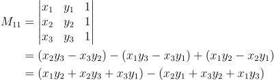
$\begin{align*} M_{11} &= \begin{vmatrix} x_1 & y_1 & 1 \\ x_2 & y_2 & 1 \\ x_3 & y_3 & 1 \\ \end{vmatrix} \\ &= (x_2y_3 - x_3y_2) - (x_1y_3 - x_3y_1) + (x_1y_2 - x_2y_1) \\ &= (x1y_2 + x_2y_3 + x_3y_1) - (x_2y_1 + x_3y_2 + x_1y_3) \end{align*}$

Having gone to the effort of finding a nice expression for M₁₁ we can reuse it to find M₁₂ by the substitution

$x_i \to s_i \equiv x_i^2 + y_i^2$

as follows:

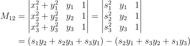
$\begin{align*} M_{12} &= \begin{vmatrix} x_1^2 + y_1^2 & y_1 & 1 \\ x_2^2 + y_2^2 & y_2 & 1 \\ x_3^2 + y_3^2 & y_3 & 1 \\ \end{vmatrix} = \begin{vmatrix} s_1^2 & y_1 & 1 \\ s_2^2 & y_2 & 1 \\ s_3^2 & y_3 & 1 \\ \end{vmatrix} \\ &= (s_1y_2 + s_2y_3 + s_3y_1) - (s_2y_1 + s_3y_2 + s_1y_3) \end{align*}$

And we can find M₁₃ from M₁₂ by reversing the role of the xs and ys.

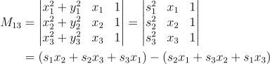
$\begin{align*} M_{13} &= \begin{vmatrix} x_1^2 + y_1^2 & x_1 & 1 \\ x_2^2 + y_2^2 & x_2 & 1 \\ x_3^2 + y_3^2 & x_3 & 1 \\ \end{vmatrix} = \begin{vmatrix} s_1^2 & x_1 & 1 \\ s_2^2 & x_2 & 1 \\ s_3^2 & x_3 & 1 \\ \end{vmatrix} \\ &= (s_1x_2 + s_2x_3 + s_3x_1) - (s_2x_1 + s_3x_2 + s_1x_3) \end{align*}$

Now we have concrete expressions for M₁₁, M₁₂, and M₁₃, and these give us concrete expressions for x₀ and y₀.

To find the radius of the circle we simply find the distance from the center (x₀, y₀) to any of the points on the circle, say (x₁, y₁).

The following Python code incorporates the derivation above.

    def circle_thru_pts(x1, y1, x2, y2, x3, y3):
        s1 = x1**2 + y1**2
        s2 = x2**2 + y2**2
        s3 = x3**2 + y3**2
        M11 = x1*y2 + x2*y3 + x3*y1 - (x2*y1 + x3*y2 + x1*y3)
        M12 = s1*y2 + s2*y3 + s3*y1 - (s2*y1 + s3*y2 + s1*y3)
        M13 = s1*x2 + s2*x3 + s3*x1 - (s2*x1 + s3*x2 + s1*x3)
        x0 =  0.5*M12/M11
        y0 = -0.5*M13/M11
        r0 = ((x1 - x0)**2 + (y1 - y0)**2)**0.5
        return (x0, y0, r0)

The code doesn’t use any loops or arrays, so it ought to be easy to port to any programming language.

For some inputs the value of M₁₁ can be (nearly) zero, in which case the three points (nearly) lie on a line. In practice M₁₁ can be nonzero and yet zero for practical purposes and so that’s something to watch out for when using the code.

The determinant at the top of the post is zero when the points are colinear. There’s a way to make rigorous the notion that in this case the points line on a circle centered at infinity.

Update: Equation of an ellipse or hyperbola through five points

Similar triangles and complex numbers

Posted on 5 June 2023 by John

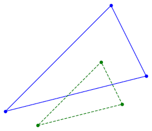
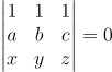
Suppose the vertices of two triangles are given by complex numbers a, b, c and x, y, z. The two triangles are similar if

$\left| \begin{matrix} 1 & 1 & 1 \\ a & b & c \\ x & y & z \\ \end{matrix} \right| = 0$

This can be found in G. H. Hardy’s classic A Course of Pure Mathematics. It’s on page 93 in the 10th edition.

Corollary

The theorem above generalizes a result from an earlier post giving a test for whether points determine an equilateral triangle. A triangle ABC is equilateral if it is similar to BCA. For triangles to be similar, corresponding vertex angles must be equal. If you can rotate the order of the angles in one triangle and the two triangles remain similar, the angles must all be equal.

Proof

Hardy’s proof of the equation above is direct and terse. I’ll quote it here in its entirety.

The condition required is that

$\overline{AB}\,/\,\overline{AC} = \overline{XY}\,/\,\overline{XZ}$

(large letters denoting the points whose arguments are the corresponding small letters), or

which is the same as the condition given.

Commentary

To expand on this a little bit, Hardy is saying that we need to show that if we take two corresponding vertices, A and X, the ratio of the lengths of corresponding sides is the same in both triangles. If memory serves, this is called the “SAS postulate.”

The determinant condition implies the last equation in Hardy’s proof. This is not obvious, but it’s easy to work out with pencil and paper. The reader may be left thinking “OK, I can see it’s true, but why would anyone think of that?” A more motivated derivation would require more background than the reader of the book is presumed to have.

You might object that Hardy’s last equation is a ratio of complex numbers, not a ratio of lengths. But you can take the absolute value of both sides. And the absolute value of a fraction is the absolute value of the numerator divided by the absolute value of the denominator. And now you’re taking a ratio of side lengths. In symbols,

$\frac{b-a}{c-a} = \frac{y-x}{z-x} \implies \frac{|b-a|}{|c-a|} = \frac{|y-x|}{|z-x|}$

Comparing approximations for ellipse perimeter

Posted on 28 May 2023 by John

This post will compare the accuracy of approximations for the perimeter of an ellipse.

The exact perimeter is given in terms of an elliptic integral. (That’s where the elliptic integrals gets their name.) And so an obvious way to approximate the perimeter would be to expand the elliptic integral in a power series. Unfortunately this series converges slowly for highly eccentric ellipses.

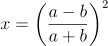
Ernst Kummer found a series that converges more quickly [1]. Let a and b be the semi-major and semi-minor axes of an ellipse and let

$x = \left(\frac{a-b}{a+b} \right )^2$

Then Kummer’s series is

$\pi(a+b)\left(1 + \frac{x}{4} + \frac{x^2}{64} + \frac{x^3}{256} + \frac{25x^4}{16384} + \cdots \right )$

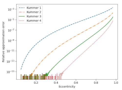
The following plot compares the accuracy of truncating Kummer’s series after powers of x equal to 1 through 4.

The noise at the bottom of the chart comes from the limits of machine precision. For moderate values of eccentricity, three terms of Kummer’s series gives an approximation so accurate that all the error is coming from the limitations of floating point resolution.

I’ve written about approximations for the perimeter of an ellipse before. The approximation based on the 3/2 norm is about as accurate as Kummer’s series truncated after the x term. The error in Ramanujan’s approximation is between that of Kummer’s series with the cubic and quartic terms.

For the orbit of Pluto (e = 0.2488) the first-order Kummer approximation is good to 9 figures and the higher-order approximations are essentially good to machine precision.

For the orbit of Haley’s comet (e = 0.9671) the successive Kummer approximations are good to 2, 3, 4, and 5 figures.

[1] Carl E. Linderholm and Arthur C. Segal. An Overlooked Series for the Elliptic Perimeter. Mathematics Magazine, Vol. 68, No. 3 (Jun., 1995), pp. 216–220.

Contraharmonic mean

Posted on 20 May 2023 by John

I’ve mentioned the harmonic mean multiple times here, most recently last week. The harmonic mean pops up in many contexts.

The contraharmonic mean is a variation on the harmonic mean that comes up occasionally, though not as often as its better known sibling.

Definition

The contraharmonic mean of two positive numbers a and b is

$C = \frac{a^2 + b^2}{a + b}$

and more generally, the contraharmonic mean of a sequence of positive numbers is the sum of their squares over their sum.

Why the name?

What is “contra” about the contraharmonic mean? The harmonic mean and contraharmonic mean have a sort of reciprocal relationship. The ratio

$\frac{a - m}{m - b}$

equals a/b when m is the harmonic mean and it equals b/a when m is the contraharmonic mean.

Geometric visualization

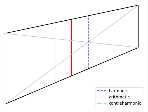
Construct a trapezoid with two vertical sides, one of length a and another of length b. The vertical slice through the intersection of the diagonals, the dashed blue line in the diagram below, has length equal to the harmonic mean of a and b.

The vertical slice midway between the two vertical sides, the solid red line in the diagram, has length equal to the arithmetic mean of a and b.

The vertical slice on the opposite side of the red line, as from the red line on one side as the blue line is on the other, the dash-dot green line above, has length equal to the contraharmonic mean of a and b.

Connection to statistics

The contraharmonic mean of a list of numbers is the ratio of the sum of the squares to the sum. If we divide the numerator and denominator by the number of terms n we see this is the ratio of the second moment to the first moment, i.e. the mean of the squared values divided the mean of the values.

This smells like the ratio of variance to mean, known as the index of dispersion D, except variance is the second central moment rather than the second moment. The second moment equals variance plus the square of the mean, and so

$D = \frac{\sigma^2}{\mu}$

and

$C = \frac{\text{E}(X^2)}{\text{E}(X)} = \frac{\sigma^2 + \mu^2}{\mu} = D + \mu.$

How Albrecht Dürer drew an 11-sided figure

Posted on 14 April 2023 by John

You cannot exactly construct an 11-sided regular polygon (called a hendecagon or an undecagon) using only a straight edge and compass. Gauss fully classified which regular n-gons can be constructed, and this isn’t one of them [1].

However, Albrecht Dürer [2] came up with a good approximate construction for a hendecagon.

To construct an eleven-sided figure by means of a compass, I take a quarter of a circle’s diameter, extend it by one eighth of its length, and use this for the construction of the eleven-sided figure.

It took some trial and error for me to understand what Dürer meant.

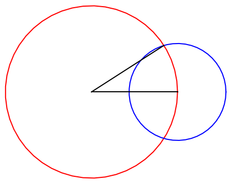
In more explicit terms, draw a circle of radius R centered at the origin. Then draw a circle of radius 9R/16 centered at (R, 0). Then draw a line from the origin to the intersection of the two circles. (There are two intersections, and it doesn’t matter which one you pick.) Then this line makes an angle of approximately (360/11) degrees with the x-axis.

Without loss of generality we can assume R = 1. A point at the intersection of both circles satisfies the equation of each circle, and from these two equations in two unknowns we can determine that the x coordinate of the two intersection points is 431/512. We can then use the Pythagorean theorem to solve for y and find the inverse tangent of y/x. This shows that we’ve constructed an angle of 32.6696°. We were after an angle of 32.7272°, and so the relative error in Dürer’s approximation is less than 0.2%.

Diagram of Durer's construction

To be even more explicit, here is the Python code that created the image above.

    import matplotlib.pyplot as plt
    from numpy import linspace, sin, cos, pi

    r = 9/16
    t = linspace(0, 2*pi)
    plt.plot(cos(t), sin(t), 'r-')
    plt.plot(r*cos(t) + 1, r*sin(t), 'b-')

    x = 431/512
    y = (1 - x*x)**0.5
    plt.plot([0, 1], [0, 0], 'k')
    plt.plot([0, x], [0, y], 'k')

    plt.gca().set_aspect("equal")
    plt.axis("off")
    plt.savefig("durer11.png")

More Dürer posts

[1] The Guass-Wantzel theorem says a regular n-gon can be constructed with straight edge and compass if n factors into a power of 2 and distinct Fermat primes.

[2] I found this in A Panoply of Polygons which in turn cites “The Polygons of Albrecht Durer -1525” By Gordon Hughes, available on arXiv.

A pentagon, hexagon, and decagon walk into a bar …

Posted on 14 April 2023 by John

The new book A Panoply of Polygons cites a theorem Euclid (Proposition XIII.10) saying

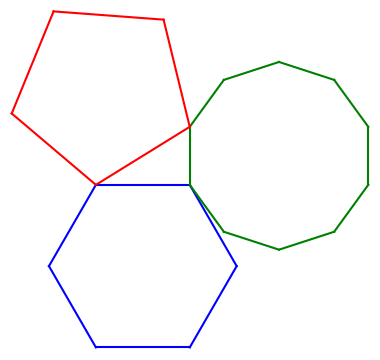
If a regular pentagon, a regular hexagon, and a regular decagon are inscribed in congruent circles, then their side lengths form a right triangle.

This isn’t exactly what Euclid said, but it’s an easy deduction from what he did say.

Here’s an illustration.

Illustrating Euclid Proposition XIII.10

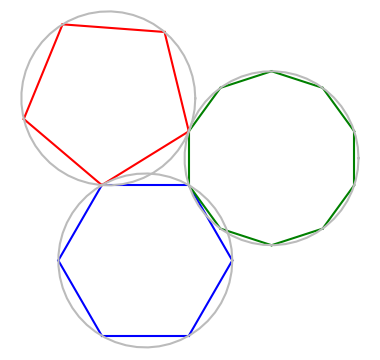
Update: Ralph Corderoy suggested in the comments that it would be good to add the congruent circles through the polygon vertices. Here is a graphic with the circles added.

Illustrating Euclid Proposition XIII.10

Connection with golden ratio

I learned about this theorem from the book cited above, which arrived in the mail yesterday. The figure looked familiar because Cliff Pickover had posted essentially the same illustration on Twitter recently, saying that not only is there a right triangle in the middle of the diagram, this triangle is half of a golden rectangle.

The length of the side of a regular polygon with n sides is 2R sin(π/n) where R is the radius of the circle through the vertices. So to prove that the ratio between the side of the hexagon and the side of the decagon is the golden ratio φ, it suffices to prove

sin(π/6) / sin(π/10) = φ

You could verify this in Mathematica by seeing that the following returns True.

    Sin[Pi/6]/ Sin[Pi/10] == GoldenRatio

Python code

Here’s the code I used to create the image above.

    from numpy import exp, pi, arange
    import matplotlib.pyplot as plt
    
    # Vertices of a hexagon
    hexa = exp(2j*pi*arange(6)/6)
    
    # Vertices of a decagon, shifted and rotated
    # to have a side perpendicular to the hexagon
    deca = exp(2j*pi*(0.5+arange(10))/10)
    deca += hexa[1] - deca[5]
    
    # Shift and rotate a pentagon to share one vertex 
    # with the hexagon and one vertex with the decagon
    omega = exp(2j*pi/5)
    c = (hexa[2]*omega - deca[4])/(omega - 1)
    penta = c + (hexa[2] - c)*exp(2j*pi*arange(5)/5) 
    
    def connect(p, q, c):
        plt.plot([p.real, q.real], [p.imag, q.imag], '-', color=c)
    
    plt.gca().set_aspect("equal")
    
    for n in range(-1, 5):
        connect(hexa[n], hexa[n+1], 'blue')
    for n in range(-1, 9):
        connect(deca[n], deca[n+1], 'green')
    for n in range(-1, 4):
        connect(penta[n], penta[n+1], 'red')
    
    plt.show()

The ability to use −1 to as the index to the last element of an array simplifies the code that connects the vertices. In a language like C you’d have to write an extra statement after your loop to join the last vertex to the first.

When I first saw the illustration in Panoply of Pentagons I though that the top of the pentagon was parallel to the top of the hexagon. When I wrote the Python code first assuming this orientation of the pentagon, things didn’t line up. Writing the code made me pay closer attention, as is often the case.

A new trig identity

Posted on 13 April 2023 by John

This evening I ran across a trig identity I hadn’t seen before. I doubt it’s new to the world, but it’s new to me.

Let A, B, and C be the angles of an arbitrary triangle. Then

sin² A + sin² B + sin² C = 2 + 2 cos A cos B cos C.

This looks a little like the Pythagorean theorem, but the Pythagorean theorem involves the sides of a triangle, not the angles. (I expect there’s an interesting generalization of the identity above to spherical geometry where sides are angles.)

This identity also looks a little like the law of cosines, but the law of cosines mixes sides and angles, and this identity only involves angles.

Source: Lemma 4.4.3 in A Panoply of Polygons by Claudi Alsina and Roger B. Nelsen.

Double duals of polyhedra

Posted on 6 April 2023 by John

The previous post mentioned the dual of a tetrahedron is another tetrahedron. The dual of a cube is an octahedron and the dual of an octahedron is a cube. And the dual of a dodecahedron is an icosahedron, and the dual of an icosahedron is a dodecahedron.

So if you take the dual of a regular solid twice, you get back another regular solid of the same type. But you do not get the same regular solid back. To see this, let’s look at how you form the dual of a polyhedron.

To find the dual of a polyhedron, you make a new polyhedron whose vertices are the centroids of the faces of the original polyhedron. The vertices of a regular polyhedron all lie on the surface of a sphere. A face of the polygon lies inside the sphere, so the centroids of the solid are all inside the sphere. Since the centroids form the vertices of a regular solid, they also all lie on a sphere, but a smaller sphere inside the first sphere.

Size of duals

If you take the double dual of a regular solid, the dual of the dual, then you get a smaller solid of the same type. How much smaller? We can get Mathematica to calculate this for us.

The function DualPolyhedron does what the name implies. Let’s apply this to the default tetrahedron. When we enter

    DualPolyhedron[ Tetrahedron[] ]

we get back

    Tetrahedron[{2 Pi/3}, Pi}, 1/3]

The default tetrahedron, returned by calling Tetrahedron[], has vertices

(1, 0, 0)
(0, 0, 1)
(1, 0, 1)
(1, 1, 1)

Each edge has length 1. Its dual has been rotated by 2π/3 about the z axis and by π about the y axis, and has edges of length 1/3. Taking the dual of a tetrahedron rotates the tetrahedron and shrinks it by a factor of 3 (in each dimension).

Size of double duals

If we take the double dual of a tetrahedron, we get a tetrahedron nine times smaller. Let’s see what happens to the rest of the regular solids.

    DualPolyhedron[DualPolyhedron[#]] & /@ 
        {Tetrahedron[], Octahedron[], Cube[],
         Dodecahedron[], Icosahedron[]}

This tells us again what we found above for the double dual of a tetrahedron. It also tells us that taking the double dual of an octahedron or cube results in an octahedron or cube 3 times smaller. And it tells us that taking the double dual of a dodecahedron or icosahedron reduces its size by a factor of

(5 + 2√ 5)/15 = 0.6314…

Taking the double dual shrinks a regular solid, and the amount of shrinkage goes down as the number of faces goes up.

Orientation of double duals

The process of taking the double dual may also rotate the solid. The second dual of the standard tetrahedron, for example, is not just 9 times smaller. It’s also been rotated. We can see this by calling PolyhedronCoordinates. The code

    PolyhedronCoordinates[ 
        DualPolyhedron[ DualPolyhedron[ Tetrahedron[] ] ] ]

shows that the new vertices are

(7/9, 2/9, 6/9)
(7/9, 2/9, 7/9)
(7/9, 3/9, 7/9)
(6/9, 2/9, 7/9)

So the second dual of the tetrahedron is not just 9 times smaller.

However, taking the double dual of the rest of the regular solids does not change the orientation. You could verify this for the cube and dodecahedron using Mathematica. It then follows that taking the double dual of octahedra and icosahedra does not change the orientation.

Sixth dual

If you take the dual of a tetrahedron 6 times you do return to the original orientation, but not if you take the dual fewer times. You can verify this by running the following:

    NestList[DualPolyhedron, Tetrahedron[], 6]

Solid angle of a star

Posted on 20 March 2023 by John

The apparent size of a distant object can be measured by projecting the object onto a unit sphere around the observer and calculating the area of the projected image.

A unit sphere has area 4π. If you’re in a ship far from land, the solid angle of the sky is 2π steradians because it takes up half a sphere.

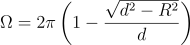
If the object you’re looking at is a sphere of radius r whose center is a distance d away, then its apparent size is

$\Omega = 2\pi\left(1 - \frac{\sqrt{d^2 - r^2}}{d}\right)$

steradians. This formula assumes d > r. Otherwise you’re not looking out at the sphere; you’re inside the sphere.

If you’re looking at a star, then d is much larger than r, and we can simplify the equation above. The math is very similar to the math in an earlier post on measuring tapes. If you want to measure the size of a room, and something is blocking you from measuring straight from wall to wall, it doesn’t make much difference if the object is small relative to the room. It all has to do with Taylor series and the Pythagorean theorem.

Think of the expression above as a function of r and expand it in a Taylor series around r = 0.

$\Omega = 2\pi\left(1 - \frac{\sqrt{d^2 - r^2}}{d}\right) = 2\pi\left(\frac{\sqrt{r^2}}{2d^2} + \frac{r^4}{8d^4} + \cdots \right)$

and so

$\Omega \approx \frac{\pi r^2}{d^2}$

with an error on the order of (r/d)⁴. To put it another way, the error in our approximation for Ω is on the order of Ω². The largest object in the sky is the sun, and it has apparent size less than 10⁻⁴, so Ω is always small when looking at astronomical objects, and Ω² is negligible.

So for practical purposes, the apparent size of a celestial object is π times the square of the ratio of its radius to its distance. This works fine for star gazing. The approximation wouldn’t be as accurate for watching a hot air balloon launch up close.

Square degrees

Sometimes solid angles are measured in square degrees, given by π/4 times the square of the apparent diameter in degrees. This implicitly uses the approximation above since the apparent radius is r/d.

(The area of a square is diameter squared, and a circle takes up π/4 of a square.)

Examples

When I typed

    3.1416 (radius of sun / distance to sun)^2

into Wolfram Alpha I got 6.85 × 10⁻⁵. (When I used “pi” rather than 3.1416 it interpreted this as the radius of a pion particle.)

When I typed

    3.1416 (radius of moon / distance to moon)^2

I got 7.184 × 10⁻⁵, confirming that the sun and moon are approximately the same apparent size, which makes a solar eclipse possible.

The brightest star in the night sky is Sirius. Asking Wolfram Alpha

    3.1416 (radius of Sirius / distance to Sirius)^2

we get 6.73 × 10⁻¹⁶.

Geometry

A parabola, a triangle, and a circle

Equation of a circle through three points

Similar triangles and complex numbers

Corollary

Proof

Commentary

Related posts

Comparing approximations for ellipse perimeter

Contraharmonic mean

Definition

Why the name?

Geometric visualization

Connection to statistics

How Albrecht Dürer drew an 11-sided figure

More Dürer posts

A pentagon, hexagon, and decagon walk into a bar …

Connection with golden ratio

Python code

Related posts

A new trig identity

Double duals of polyhedra

Size of duals

Size of double duals

Orientation of double duals

Sixth dual

Related posts

Solid angle of a star

Square degrees

Examples

Related posts