I haven’t been able to find technical details of the orbit of Artemis I, and some of what I’ve found has been contradictory, but here are some back-of-the-envelope calculations based on what I’ve pieced together. If someone sends me better information I can update this post.
Artemis is in a highly eccentric orbit around the moon, coming within 130 km (80 miles) of the moon’s surface at closest pass, and this orbit will take 14 days to complete. The weak link in this data is “14 days.” Surely this number has been rounded for public consumption.
If we assume Artemis is in a Keplerian orbit, i.e. we can ignore the effect of the Earth, then we can calculate the shape of the orbit using the information above. This assumption is questionable because as I understand it the reason for such an eccentric orbit has something to do with Lagrange points, which means the Earth’s gravity matters. Still, I image the effect of Earth’s gravity is a smaller source of error than the lack of accuracy in knowng the period.
Solving for axes
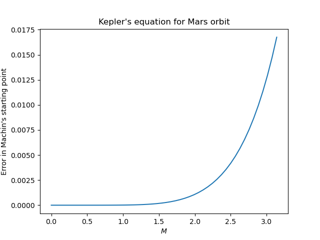
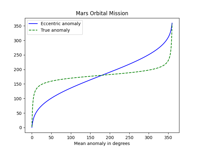
Artemis is orbiting the moon similarly to how the Mars Orbiter Mission orbited Mars. We can use Kepler’s equation for period T to solve for the semi-major axis a of the orbit.
T = 2π √(a³/μ)
Here μ = GM, with G being the gravitational constant and M being the mass of the moon. Now
G = 6.674 × 10⁻¹¹ N m²/kg²
and
M = 7.3459 × 10²² kg.
If we assume T is 14 × 24 × 3600 seconds, then we get
a = 56,640 km
or 35,200 miles. The value of a is rough since the value of T is rough.
Assuming a Keplerian orbit, the moon is at one focus of the orbit, located a distance c from the center of the ellipse. If Artemis is 130 km from the surface of the moon at perilune, and the radius of the moon is 1737 km, then
c = a − (130 + 1737) km = 54,770 km
or 34,000 miles. The semi-minor axis b satisfies
b² = a² − c²
and so
b = 14,422 km
or 8962 miles.
Orbit shape
The eccentricity is c/a = 0.967. As I’ve written about before, eccentricity is hard to interpret intuitively. Aspect ratio is much easier to imaging than eccentricity, and the relation between the two is highly nonlinear.
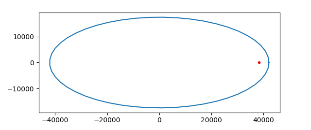
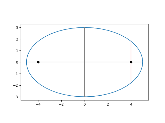
Assuming everything above, here’s what the orbit would look like. The distances on the axes are in kilometers.
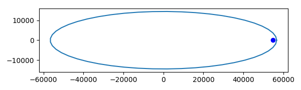
The orbit is highly eccentric: the center of the orbit is far from the foci of the orbit. But the aspect ratio is about 1/4. The orbit is only about 4 times wider in one direction than the other. It’s obviously an ellipse, but it’s not an extremely thin ellipse.
Lagrange points
In an earlier post I showed how to compute the Lagrange points for the Sun-Earth system. We can use the same equations for the Earth-Moon system.
The equations for the distance r from the Lagrange points L1 and L2 to the moon are
![]()
The equation for L1 corresponds to taking ± as − and the equation for L2 corresponds to taking ± as +. Here M1 and M2 are the masses of the Earth and Moon respectively, and R is the distance between the two bodies.
If we modify the code from the earlier post on Lagrange points we get
L1 = 54784 km
L2 = 60917 km
where L1 is on the near side of the moon and L2 on the far side. We estimated the semi-major axis a to be 56,640 km. This is about 3% larger than the distance from the moon to L1. So the orbit of Artemis passes near or through L1. This assumes the axis of the Artemis orbit is aligned with a line from the moon to Earth, which I believe is at least approximately correct.