Random minimum spanning trees

Posted on 9 August 2017 by John

I just ran across a post by John Baez pointing to an article [the link has gone away] by Alan Frieze on random minimum spanning trees.

Here’s the problem.

Create a complete graph with n nodes, i.e. connect every node to every other node.
Assign each edge a uniform random weight between 0 and 1.
Find the minimum spanning tree.
Add up the edges of the weights in the minimum spanning tree.

The surprise is that as n goes to infinity, the expected value of the process above converges to the Riemann zeta function at 3, i.e.

ζ(3) = 1/1³ + 1/2³ + 1/3³ + …

Incidentally, there are closed-form expressions for the Riemann zeta function at positive even integers. For example, ζ(2) = π² / 6. But no closed-form expressions have been found for odd integers.

Simulation

Here’s a little Python code to play with this.

    import networkx as nx
    from random import random

    N = 1000

    G = nx.Graph()
    for i in range(N):
        for j in range(i+1, N):
            G.add_edge(i, j, weight=random())

    T = nx.minimum_spanning_tree(G)
    edges = T.edges(data=True)

    print( sum( e[2]["weight"] for e in edges ) )

When I ran this, I got 1.2307, close to ζ(3) = 1.20205….

I ran this again, putting the code above inside a loop, averaging the results of 100 simulations, and got 1.19701. That is, the distance between my simulation result and ζ(3) went from 0.03 to 0.003.

There are two reasons I wouldn’t get exactly ζ(3). First, I’m only running a finite number of simulations (100) and so I’m not computing the expected value exactly, but only approximating it. (Probably. As in PAC: probably approximately correct.) Second, I’m using a finite graph, of size 1000, not taking a limit as graph size goes to infinity.

My limited results above suggest that the first reason accounts for most of the difference between simulation and theory. Running 100 replications cut the error down by a factor of 10. This is exactly what you’d expect from the central limit theorem. This suggests that for graphs as small as 1000 nodes, the expected value is close to the asymptotic value.

You could experiment with this, increasing the graph size and increasing the number of replications. But be patient. It takes a while for each replication to run.

Generalization

The paper by Frieze considers more than the uniform distribution. You can use any non-negative distribution with finite variance and whose cumulative distribution function F is differentiable at zero. The more general result replaces ζ(3) with ζ(3) / F ‘(0). We could, for example, replace the uniform distribution on weights with an exponential distribution. In this case the distribution function is 1 − exp(−x), at its derivative at the origin is 1, so our simulation should still produce approximately ζ(3). And indeed it does. When I took the average of 100 runs with exponential weights I got a value of 1.2065.

There’s a little subtlety around using the derivative of the distribution at 0 rather than the density at 0. The derivative of the distribution (CDF) is the density (PDF), so why not just say density? One reason would be to allow the most general probability distributions, but a more immediate reason is that we’re up against a discontinuity at the origin. We’re looking at non-negative distributions, so the density has to be zero to the left of the origin.

When we say the derivative of the distribution at 0, we really mean the derivative at zero of a smooth extension of the distribution. For example, the exponential distribution has density 0 for negative x and density exp(−x) for non-negative x. Strictly speaking, the CDF of this distribution is 1 − exp(−x) for non-negative x and 0 for negative x. The left and right derivatives are different, so the derivative doesn’t exist. By saying the distribution function is simply exp(−x), we’ve used a smooth extension from the non-negative reals to all reals.

Nearly all the area in a high-dimensional sphere is near the equator

Posted on 13 July 2017 by John

Nearly all the area of a high-dimensional sphere is near the equator. And by symmetry, it doesn’t matter which equator you take. Draw any great circle and nearly all of the area will be near that circle. This is the canonical example of “concentration of measure.”

What exactly do we mean by “nearly all the area” and “near the equator”? You get to decide. Pick your standard of “nearly all the area,” say 99%, and your definition of “near the equator,” say within 5 degrees. Then it’s always possible to take the dimension high enough that your standards are met. The more demanding your standard, the higher the dimension will need to be, but it’s always possible to pick the dimension high enough.

This result is hard to imagine. Maybe a simulation will help make it more believable.

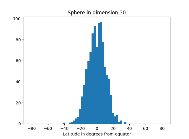
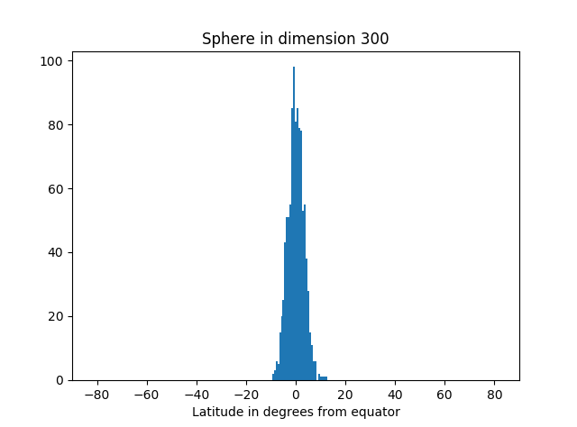
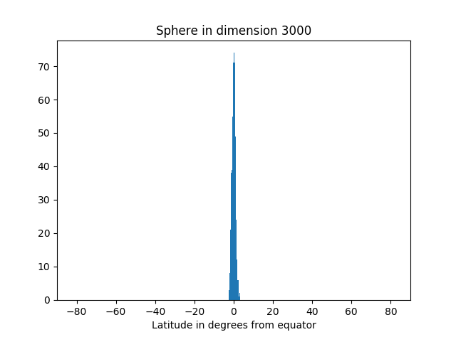
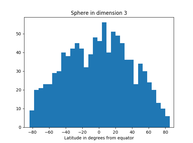
In the simulation below, we take as our “north pole” the point (1, 0, 0, 0, …, 0). We could pick any unit vector, but this choice is convenient. Our equator is the set of points orthogonal to the pole, i.e. that have first coordinate equal to zero. We draw points randomly from the sphere, compute their latitude (i.e. angle from the equator), and make a histogram of the results.

The area of our planet isn’t particularly concentrated near the equator.

But as we increase the dimension, we see more and more of the simulation points are near the equator.

Here’s the code that produced the graphs.

from scipy.stats import norm
from math import sqrt, pi, acos, degrees
import matplotlib.pyplot as plt

def pt_on_sphere(n):
    # Return random point on unit sphere in R^n.
    # Generate n standard normals and normalize length.
    x = norm.rvs(0, 1, n)
    length = sqrt(sum(x**2))
    return x/length

def latitude(x):
    # Latitude relative to plane with first coordinate zero.
    angle_to_pole = acos(x[0]) # in radians
    latitude_from_equator = 0.5*pi - angle_to_pole
    return degrees( latitude_from_equator )

N = 1000 # number of samples

for n in [3, 30, 300, 3000]: # dimension of R^n
    
    latitudes = [latitude(pt_on_sphere(n)) for _ in range(N)]
    plt.hist(latitudes, bins=int(sqrt(N)))
    plt.xlabel("Latitude in degrees from equator")
    plt.title("Sphere in dimension {}".format(n))
    plt.xlim((-90, 90))
    plt.show()

Not only is most of the area near the equator, the amount of area outside a band around the equator decreases very rapidly as you move away from the band. You can see that from the histograms above. They look like a normal (Gaussian) distribution, and in fact we can make that more precise.

If A is a band around the equator containing at least half the area, then the proportion of the area a distance r or greater from A is bound by exp( −(n − 1)r² ). And in fact, this holds for any set A containing at least half the area; it doesn’t have to be a band around the equator, just any set of large measure.

Simple random number generator does surprisingly well

Posted on 5 July 2017 by John

I was running the NIST statistical test suite recently. I wanted an example of a random number generator where the tests failed, and so I used a simple generator, a linear congruence generator. But to my surprise, the generator passed nearly all the tests, even though some more sophisticated generators failed some of the same tests. This says more about the NIST test suite than it says about the LCG being tested.

This post will implement a couple of the simplest tests in Python and show that the generator does well.

The linear congruential generator used here starts with an arbitrary seed, then at each step produces a new number by multiplying the previous number by a constant and taking the remainder by 2³¹ – 1. The multiplier constant was chosen to be one of the multipliers recommended in [1].

We’ll need a couple math functions:

from math import sqrt, log

and we need to define the constants for our generator.

# Linear congruence generator (LCG) constants
z = 20170705   # seed
a = 742938285  # multiplier
e = 31         # will need this later
m = 2**e -1    # modulus

Next we form a long string of 0’s and 1’s using our generator

# Number of random numbers to generate
N = 100000     

# Format to print bits, padding with 0's on the left if needed
formatstr = "0" + str(e) + "b"

bit_string = ""
for _ in range(N):
    z = a*z % m # LCG
    bit_string += format(z, formatstr)

Next we run a couple tests. First, we count the number of 1’s in our string of bits. We expect about half the bits to be 1’s. We can quantify “about” as within two standard deviations.

def count_ones(string):
    ones = 0
    for i in range(len(string)):
        if string[i] == '1':
            ones += 1
    return ones

ones = count_ones(bit_string)
expected = e*N/2
sd = sqrt(0.25*N)
print( "Number of 1's: {}".format(ones) )
print( "Expected: {} to {}".format(expected - 2*sd, expected + 2*sd) )

The results are nothing unusual:

Number of 1's: 1550199
Expected: 1549683.8 to 1550316.2

Next we look at the length of the longest runs on 1’s. I’ve written before about the probability of long runs and the code below uses a couple results from that post.

def runs(string):
    max_run = 0
    current_run = 0
    for i in range(len(string)):
        if string[i] == '1':
            current_run += 1
        else:
            current_run = 0
        max_run = max(max_run, current_run)
    return max_run

runlength = runs(bit_string)
expected = -log(0.5*e*N)/log(0.5)
sd = 1/log(2)
print( "Run length: {}".format(runlength) )
print( "Expected: {} to {}".format(expected - 2*sd, expected + 2*sd) )

Again the results are nothing unusual:

Run length: 19
Expected: 17.7 to 23.4

Simple random number generators are adequate for many uses. Some applications, such as high dimensional integration and cryptography, require more sophisticated generators, but sometimes its convenient and sufficient to use something simple. For example, code using the LCG generator above would be easier to debug than code using the Mersenne Twister. The entire state of the LCG is a single number, whereas the Mersenne Twister maintains an internal state of 312 numbers.

One obvious limitation of the LCG used here is that it couldn’t possibly produce more than 2³¹ – 1 values before repeating itself. Since the state only depends on the last value, every time it comes to a given output, the next output will be whatever the next output was the previous time. In fact, [1] shows that it does produce 2³¹ – 1 values before cycling. If the multiplier were not chosen carefully it could have a shorter period.

So our LCG has a period of about two billion values. That’s a lot if you’re writing a little game, for example. But it’s not enough for many scientific applications.

* * *

[1] George S. Fishman and Louis R. Moore III, An exhaustive analysis of multiplicative congruential random number generators with modulus 2³¹ – 1, SIAM Journal of Scientific and Statistical Computing, Vol. 7, no. 1, January 1986.

Polynomials evaluated at integers

Posted on 21 June 2017 by John

Let p(x) = a₀ + a₁x + a₂x² + … + a_nxⁿ and suppose at least one of the coefficients a_i is irrational for some i ≥ 1. Then a theorem by Weyl says that the fractional parts of p(n) are equidistributed as n varies over the integers. That is, the proportion of values that land in some interval is equal to the length of that interval.

Clearly it’s necessary that one of the coefficients be irrational. What may be surprising is that it is sufficient.

If the coefficients are all rational with common denominator N, then the sequence would only contain multiples of 1/N. The interval [1/3N, 2/3N], for example, would never get a sample. If a₀ were irrational but the rest of the coefficients were rational, we’d have the same situation, simply shifted by a₀.

This is a theorem about what happens in the limit, but we can look at what happens for some large but finite set of terms. And we can use a χ² test to see how evenly our sequence is compared to what one would expect from a random sequence.

In the Python code below, we use the polynomial p(x) = √2 x² + πx + 1 and evaluate p at 0, 1, 2, …, 99,999. We then count how many fall in the bins [0, 0.01), [0.01, 0.02), … [0.99, 1] and compute a chi-square statistic on the counts.

from math import pi, sqrt, floor

def p(x):
    return 1 + pi*x + sqrt(2)*x*x

def chisq_stat(O, E):
    return sum( (o - e)**2/e for (o, e) in zip(O, E) )

def frac(x):
    return x - floor(x)

N = 100000
data = [frac(p(n)) for n in range(N)]

count = [0]*100
for d in data:
    count[ int(floor(100*d)) ] += 1

expected = [N/100]*100

print(chisq_stat(count, expected))

We get a chi-square statistic of 95.4. Since we have 100 bins, there are 99 degrees of freedom, and we should compare our statistic to a chi-square distribution with 99 degrees of freedom. Such a distribution has mean 99 and standard deviation √(99*2) = 14.07, so a value of 95.4 is completely unremarkable.

If we had gotten a very large chi-square statistic, say 200, we’d have reason to suspect something was wrong. Maybe a misunderstanding on our part or a bug in our software. Or maybe the sequence was not as uniformly distributed as we expected.

If we had gotten a very small chi-square statistic, say 10, then again maybe we misunderstood something, or maybe our sequence is remarkably evenly distributed, more evenly than one would expect from a random sequence.

Fractional parts, invariant measures, and simulation

Posted on 18 June 2017 by John

A function f: X → X is measure-preserving if for each iteration of f sends the same amount of stuff into a given set. To be more precise, given a measure μ and any μ-measurable set E with μ(E) > 0, we have

$\mu( E ) = \mu( f^{-1}(E) )$

You can read the right side of the equation above as “the measure of the set of points that f maps into E.” You can apply this condition repeatedly to see that the measure of the set of points mapped into E after n iterations is still just the measure of E.

If X is a probability space, i.e. μ( X ) = 1, then you could interpret the definition of measure-preserving to mean that the probability that a point ends up in E after n iterations is independent of n. We’ll illustrate this below with a simulation.

Let X be the half-open unit interval (0, 1] and let f be the Gauss map, i.e.

$f(x) = \frac{1}{x} - \left\lfloor \frac{1}{x}\right\rfloor$

where [z] is the integer part of z. The function f is measure-preserving, though not for the usual Lebesgue measure. Instead it preserves the following measure:

$\mu(E) = \frac{1}{\log 2} \int_E \frac{1}{1+x} \, dx$

Let’s take as our set E an interval [a, b] and test via simulation whether the probability of landing in E after n iterations really is just the measure of E, independent of n.

We can’t just generate points uniformly in the interval (0, 1]. We have to generate the points so that the probability of a point coming from a set E is μ(E). That means the PDF of the distribution must be p(x) = 1 / (log(2) (1 + x)). We use the inverse-CDF method to generate points with this density in the Python code below.

from math import log, floor
from random import random

def gauss_map(x):
    y = 1.0/x
    return y - floor(y)

# iterate gauss map n times
def iterated_gauss_map(x, n):
    while n > 0:
        x = gauss_map(x)
        n = n - 1
    return x      

# measure mu( [a,b] )
def mu(a, b):
    return (log(1.0+b) - log(1.0+a))/log(2.0)

# Generate samples with Prob(x in E) = mu( E )
def sample():
    u = random()
    return 2.0**u - 1.0

def simulate(num_points, num_iterations, a, b):
    count = 0
    for _ in range(num_points):
        x = sample()
        y = iterated_gauss_map(x, num_iterations)
        if a < y < b:
            count += 1
    return count / num_points

# Change these parameters however you like
a, b = 0.1, 0.25
N = 1000000

exact = mu(a, b)
print("Exact probability:", exact)
print("Simulated probability after n iterations")
for n in range(1, 10):
    simulated = simulate(N, n, a, b)
    print("n =", n, ":", simulated)

Here’s the output I got:

Exact probability: 0.18442457113742736
Simulated probability after n iterations
n = 1 : 0.184329
n = 2 : 0.183969
n = 3 : 0.184233
n = 4 : 0.184322
n = 5 : 0.184439
n = 6 : 0.184059
n = 7 : 0.184602
n = 8 : 0.183877
n = 9 : 0.184834

With 1,000,000 samples, we expect the results to be the same to about 3 decimal places, which is what we see above.

Related post: Irrational rotations are ergodic.

(A transformation f is ergodic if it is measure preserving and the only sets E with f^–1(E) = E are those with measure 0 or full measure. Rational rotations are measure-preserving but not ergodic. The Gauss map above is ergodic.)

Irrational rotations are ergodic

Posted on 1 June 2017 by John

In a blog post yesterday, I mentioned that the golden angle is an irrational portion of a circle, and so a sequence of rotations by the golden angle will not repeat itself. We can say more: rotations by an irrational portion of a circle are ergodic. Roughly speaking, this means that not only does the sequence not repeat itself, the sequence “mixes well” in a technical sense.

Ergodic functions have the property that “the time average equals the space average.” We’ll unpack what that means and illustrate it by simulation.

Suppose we pick a starting point x on the circle then repeatedly rotate it by a golden angle. Take an integrable function f on the circle and form the average of its values at the sequence of rotations. This is the time average. The space average is the integral of f over the circle, divided by the circumference of the circle. The ergodic theorem says that the time average equals the space average, except possibly for a setting of starting values of measure zero.

More generally, let X be a measure space (like the unit circle) with measure μ let T be an ergodic transformation (like rotating by a golden angle), Then for almost all starting values x we have the following:

$\lim_{n\to \infty} \frac{1}{n} \sum_{k=0}^{n-1} f(T^k x) = \frac{1}{\mu(X)} \int_X f\, d\mu$

Let’s do a simulation to see this in practice by running the following Python script.

        from scipy import pi, cos
        from scipy.constants import golden
        from scipy.integrate import quad
        
        golden_angle = 2*pi*golden**-2
        
        def T(x):
            return (x + golden_angle) % (2*pi)
        
        def time_average(x, f, T, n):
            s = 0
            for k in range(n):
                s += f(x)
                x = T(x)
            return s/n
        
        def space_average(f):
            integral = quad(f, 0, 2*pi)[0]
            return integral / (2*pi)
        
        f = lambda x: cos(x)**2
        N = 1000000
        
        print( time_average(0, f, T, N) )
        print( space_average(f) )

In this case we get 0.49999996 for the time average, and 0.5 for the space average. They’re not the same, but we only used a finite value of n; we didn’t take a limit. We should expect the two values to be close because n is large, but we shouldn’t expect them to be equal.

Update: The code and results were updated to fix a bug pointed out in the comments below. I had written ... % 2*pi when I should have written ... % (2*pi). I assumed the modulo operator was lower precedence than multiplication, but it’s not. It was a coincidence that the buggy code was fairly accurate.

A friend of mine, a programmer with decades of experience, recently made a similar error. He’s a Clojure fan but was writing in C or some similar language. He rightfully pointed out that this kind of error simply cannot happen in Clojure. Lisps, including Clojure, don’t have operator precedence because they don’t have operators. They only have functions, and the order in which functions are called is made explicit with parentheses. The Python code x % 2*pi corresponds to (* (mod x 2) pi) in Clojure, and the Python code x % (2*pi) corresponds to (mod x (* 2 pi)).

Weibull distribution and Benford’s law

Posted on 2 May 2017 by John

Introduction to Benford’s law

In 1881, Simon Newcomb noticed that the edges of the first pages in a book of logarithms were dirty while the edges of the later pages were clean. From this he concluded that people were far more likely to look up the logarithms of numbers with leading digit 1 than of those with leading digit 9. Frank Benford studied the same phenomena later and now the phenomena is known as Benford’s law, or sometime the Newcomb-Benford law.

A data set follows Benford’s law if the proportion of elements with leading digit d is approximately

log₁₀((d + 1)/d).

You could replace “10” with b if you look at the leading digits in base b.

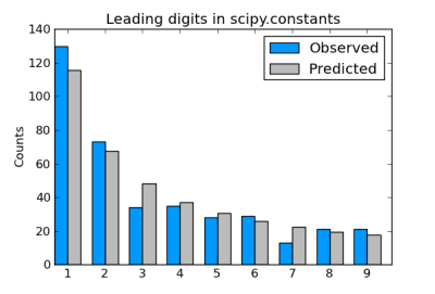
Sets of physical constants often satisfy Benford’s law, as I showed here for the constants defined in SciPy.

Incidentally, factorials satisfy Benford’s law exactly in the limit.

Weibull distributions

The Weibull distribution is a generalization of the exponential distribution. It’s a convenient distribution for survival analysis because it can have decreasing, constant, or increasing hazard, depending on whether the value of a shape parameter γ is less than, equal to, or greater than 1 respectively. The special case of constant hazard, shape γ = 1, corresponds to the exponential distribution.

Weibull and Benford

If the shape parameter of a Weibull distributions is “not too large” then samples from that distribution approximately follow Benford’s law (source). We’ll explore this statement with a little Python code.

SciPy doesn’t contain a Weibull distribution per se, but it does have support for a generalization of the Weibull known as the exponential Weibull. The latter has two shape parameters. We set the first of these to 1 to get the ordinary Weibull distribution.

      from math import log10, floor
      from scipy.stats import exponweib

      def leading_digit(x):
          y = log10(x) % 1
          return int(floor(10**y))

      def weibull_stats(gamma):

          distribution = exponweib(1, gamma)
          N = 10000
          samples = distribution.rvs(N)
          counts = [0]*10
          for s in samples:
              counts[ leading_digit(s) ] += 1

      print (counts)

Here’s how the leading digit distribution of a simulation of 10,000 samples from an exponential (Weibull with γ = 1) compares to the distribution predicted by Benford’s law.

      |---------------+----------+-----------|
      | Leading digit | Observed | Predicted |
      |---------------+----------+-----------|
      |             1 |     3286 |      3010 |
      |             2 |     1792 |      1761 |
      |             3 |     1158 |      1249 |
      |             4 |      851 |       969 |
      |             5 |      754 |       792 |
      |             6 |      624 |       669 |
      |             7 |      534 |       580 |
      |             8 |      508 |       511 |
      |             9 |      493 |       458 |
      |---------------+----------+-----------|

Looks like a fairly good fit. How could we quantify the fit so we can compare how the fit varies with the shape parameter? The most common approach is to use the chi-square goodness of fit test.

      def chisq_stat(O, E):
          return sum( (o - e)**2/e for (o, e) in zip(O, E) )

Here “O” stands for “observed” and “E” stands for “expected.” The observed counts are the counts we actually saw. The expected values are the values Benford’s law would predict:

      expected = [N*log10((i+1)/i) for i in range(1, 10)]

Note that we don’t want to pass counts to chisq_stat but counts[1:] instead. This is because counts starts with 0 index, but leading digits can’t be 0 for positive samples.

Here are the chi square goodness of fit statistics for a few values of γ. (Smaller is better.)

      |-------+------------|
      | Shape | Chi-square |
      |-------+------------|
      |   0.1 |      1.415 |
      |   0.5 |      9.078 |
      |   1.0 |     69.776 |
      |   1.5 |    769.216 |
      |   2.0 |   1873.242 |
      |-------+------------|

This suggests that samples from a Weibull follow Benford’s law fairly well for shape γ < 1, i.e. for the case of decreasing hazard.

Recreating the Vertigo poster

Posted on 14 February 2017 by John

In his new book The Perfect Shape, Øyvind Hammer shows how to create a graph something like the poster for Alfred Hitchcock’s movie Vertigo.

Poster from Hitchcock's Vertigo

Hammer’s code uses a statistical language called Past that I’d never heard of. Here’s my interpretation of his code using Python.

      import matplotlib.pyplot as plt
      from numpy import arange, sin, cos, exp
      
      i  = arange(5000)
      x1 = 1.0*cos(i/10.0)*exp(-i/2500.0)
      y1 = 1.4*sin(i/10.0)*exp(-i/2500.0)
      d  = 450.0
      vx = cos(i/d)*x1 - sin(i/d)*y1
      vy = sin(i/d)*x1 + cos(i/d)*y1
      
      plt.plot(vx, vy, "k")
      
      h = max(vy) - min(vy)
      w = max(vx) - min(vx)
      plt.axes().set_aspect(w/h)
      plt.show()

This code produces what’s called a harmonograph, related to the motion of a pendulum free to move in x and y directions:

Harmonograph

It’s not exactly the same as the movie poster, but it’s definitely similar. If you find a way to modify the code to make it closer to the poster, leave a comment below.

Approximate inverse of the gamma function

Posted on 11 February 2017 by John

The other day I ran across a blog post by Brian Hayes that linked to an article by David Cantrell on how to compute the inverse of the gamma function. Cantrell gives an approximation in terms of the Lambert W function.

In this post we’ll write a little Python code to kick the tires on Cantrell’s approximation. The post also illustrates how to do some common tasks using SciPy and matplotlib.

Here are the imports we’ll need.

      import matplotlib.pyplot as plt
      from scipy import pi, e, sqrt, log, linspace
      from scipy.special import lambertw, gamma, psi
      from scipy.optimize import root

First of all, the gamma function has a local minimum k somewhere between 1 and 2, and so it only makes sense to speak of its inverse to the left or right of this point. Gamma is strictly increasing for real values larger than k.

To find k we look for where the derivative of gamma is zero. It’s more common to work with the derivative of the logarithm of the gamma function than the derivative of the gamma function itself. That works just as well because gamma has a minimum where its log has a minimum. The derivative of the log of the gamma function is called ψ and is implemented in SciPy as scipy.special.psi. We use the function scipy.optimize.root to find where ψ is zero.

The root function returns more information than just the root we’re after. The root(s) are returned in the arrayx, and in our case there’s only one root, so we take the first element of the array:

      k = root(psi, 1.46).x[0]

Now here is Cantrell’s algorithm:

      c = sqrt(2*pi)/e - gamma(k)
      
      def L(x):
          return log((x+c)/sqrt(2*pi))
      
      def W(x):
          return lambertw(x)
      
      def AIG(x):
          return L(x) / W( L(x) / e) + 0.5

Cantrell uses AIG for Approximate Inverse Gamma.

How well goes this algorithm work? For starters, we’ll see how well it does when we do a round trip, following the exact gamma with the approximate inverse.

      x = linspace(5, 30, 100)
      plt.plot(x, AIG(gamma(x)))
      plt.show()

This produces the following plot:

We get a straight line, as we should, so next we do a more demanding test. We’ll look at the absolute error in the approximate inverse. We’ll use a log scale on the x-axis since gamma values get large quickly.

      y = gamma(x)
      plt.plot(y, x- AIG(y))
      plt.xscale("log")
      plt.show()

This shows the approximation error is small, and gets smaller as its argument increases.

Cantrell’s algorithm is based on an asymptotic approximation, so it’s not surprising that it improves for large arguments.

Fat-tailed random matrices

Posted on 29 January 2017 by John

Suppose you fill the components of a matrix with random values. How are the eigenvalues distributed?

We limit our attention to large, symmetric matrices. We fill the entries of the matrix on the diagonal and above the diagonal with random elements, then fill in the elements below the diagonal by symmetry.

If we choose our random values from a thin-tailed distribution, then Wigner’s semicircle law tells us what to expect from our distribution. If our matrices are large enough, then we expect the probability density of eigenvalues to be semicircular. To illustrate this, we’ll fill a matrix with samples from a standard normal distribution and compute its eigenvalues with the following Python code.

      import numpy as np
      import matplotlib.pyplot as plt

      N = 5000
      A = np.random.normal(0, 1, (N, N))    
      B = (A + A.T)/np.sqrt(2)
      eigenvalues = np.linalg.eigvalsh(B) 
      print(max(eigenvalues), min(eigenvalues))

      plt.hist(eigenvalues, bins=70)
      plt.show()

We first create an N by N non-symmetric matrix, then make it symmetric by adding it to its transpose. (That’s easier than only creating the upper-triangular elements.) We divide by the square root of 2 to return the variance of each component to its original value, in this case 1. The eigenvalues in this particular experiment ran from −141.095 to 141.257 and their histogram shows the expected semi-circular shape.

eigenvalue distribution with normally distributed matrix entries

Wigner’s semicircle law does not require the samples to come from a normal distribution. Any distribution with finite variance will do. We illustrate this by replacing the normal distribution with a Laplace distribution with the same variance and rerunning the code. That is, we change the definition of the matrix A to

      A = np.random.laplace(0, np.sqrt(0.5), (N, N))

and get very similar results. The eigenvalues ran from −140.886 to 141.514 and again we see a semicircular distribution.

eigenvalue distribution for matrix with entries drawn from Laplace distribution

But what happens when we draw samples from a heavy-tailed distribution, i.e. one without finite variance? We’ll use a Student-t distribution with ν = 1.8 degrees of freedom. When ν > 2 the t-distribution has variance ν/(ν − 2), but for smaller values of ν it has no finite variance. We change the definition of the matrix A to the following:

      A = np.random.standard_t(1.8, (N, N))

and now the distribution is quite different.

eigenvalue distribution for matrix with entries drawn from Student t distribution with 1.8 degrees of freedom

In this case the minimum eigenvalue was −9631.558 and the largest was 9633.853. When the matrix components are selected from a heavy-tailed distribution, the eigenvalues also have a heavier-tailed distribution. In this case, nearly all the eigenvalues are between -1000 and 1000, but the largest and smallest were 10 times larger. The eigenvalues are more variable, and their distribution looks more like a normal distribution and less like a semicircle.

The distributions for all thin-tailed symmetric matrices are the same. They have a universal property. But each heavy-tailed distribution gives rise to a different distribution on eigenvalues. With apologies to Tolstoy, thin-tailed matrices are all alike; every thick-tailed matrix is thick-tailed in its own way.

Update: As the first comment below rightfully points out, the diagonal entries should be divided by 2, not sqrt(2). Each of the off-diagonal elements of A + A^T are the sum of two independent random variables, but the diagonal elements are twice what they were in A. To put it another way, the diagonal elements are the sum of perfectly correlated random variables, not independent random variables.

I reran the simulations with the corrected code and it made no noticeable difference, either to the plots or to the range of the eigenvalues.

Python