Polynomials evaluated at integers

Let p(x) = a0 + a1x + a2x2 + … + anxn and suppose at least one of the coefficients ai is irrational for some i ≥ 1. Then a theorem by Weyl says that the fractional parts of p(n) are equidistributed as n varies over the integers. That is, the proportion of values that land in some interval is equal to the length of that interval.

Clearly it’s necessary that one of the coefficients be irrational. What may be surprising is that it is sufficient.

If the coefficients are all rational with common denominator N, then the sequence would only contain multiples of 1/N. The interval [1/3N, 2/3N], for example, would never get a sample. If a0 were irrational but the rest of the coefficients were rational, we’d have the same situation, simply shifted by a0.

This is a theorem about what happens in the limit, but we can look at what happens for some large but finite set of terms. And we can use a χ2 test to see how evenly our sequence is compared to what one would expect from a random sequence.

In the Python code below, we use the polynomial p(x) = √2 x² + πx + 1 and evaluate p at 0, 1, 2, …, 99,999. We then count how many fall in the bins [0, 0.01), [0.01, 0.02), … [0.99, 1] and compute a chi-square statistic on the counts.

from math import pi, sqrt, floor

def p(x):
    return 1 + pi*x + sqrt(2)*x*x

def chisq_stat(O, E):
    return sum( (o - e)**2/e for (o, e) in zip(O, E) )

def frac(x):
    return x - floor(x)

N = 100000
data = [frac(p(n)) for n in range(N)]

count = [0]*100
for d in data:
    count[ int(floor(100*d)) ] += 1

expected = [N/100]*100

print(chisq_stat(count, expected))

We get a chi-square statistic of 95.4. Since we have 100 bins, there are 99 degrees of freedom, and we should compare our statistic to a chi-square distribution with 99 degrees of freedom. Such a distribution has mean 99 and standard deviation √(99*2) = 14.07, so a value of 95.4 is completely unremarkable.

If we had gotten a very large chi-square statistic, say 200, we’d have reason to suspect something was wrong. Maybe a misunderstanding on our part or a bug in our software. Or maybe the sequence was not as uniformly distributed as we expected.

If we had gotten a very small chi-square statistic, say 10, then again maybe we misunderstood something, or maybe our sequence is remarkably evenly distributed, more evenly than one would expect from a random sequence.

Related math posts

Fractional parts, invariant measures, and simulation

A function f: X → X is measure-preserving if for each iteration of f sends the same amount of stuff into a given set. To be more precise, given a measure μ and any μ-measurable set E with μ(E) > 0, we have

\mu( E ) = \mu( f^{-1}(E) )

You can read the right side of the equation above as “the measure of the set of points that f maps into E.” You can apply this condition repeatedly to see that the measure of the set of points mapped into E after n iterations is still just the measure of E.

If X is a probability space, i.e. μ( X ) = 1, then you could interpret the definition of measure-preserving to mean that the probability that a point ends up in E after n iterations is independent of n. We’ll illustrate this below with a simulation.

Let X be the half-open unit interval (0, 1] and let f be the Gauss map, i.e.

f(x) = \frac{1}{x} - \left\lfloor \frac{1}{x}\right\rfloor

where [z] is the integer part of z. The function f is measure-preserving, though not for the usual Lebesgue measure. Instead it preserves the following measure:

\mu(E) = \frac{1}{\log 2} \int_E \frac{1}{1+x} \, dx

Let’s take as our set E an interval [a, b] and test via simulation whether the probability of landing in E after n iterations really is just the measure of E, independent of n.

We can’t just generate points uniformly in the interval (0, 1]. We have to generate the points so that the probability of a point coming from a set E is μ(E). That means the PDF of the distribution must be p(x) = 1 / (log(2) (1 + x)). We use the inverse-CDF method to generate points with this density in the Python code below.

from math import log, floor
from random import random

def gauss_map(x):
    y = 1.0/x
    return y - floor(y)

# iterate gauss map n times
def iterated_gauss_map(x, n):
    while n > 0:
        x = gauss_map(x)
        n = n - 1
    return x      

# measure mu( [a,b] )
def mu(a, b):
    return (log(1.0+b) - log(1.0+a))/log(2.0)

# Generate samples with Prob(x in E) = mu( E )
def sample():
    u = random()
    return 2.0**u - 1.0

def simulate(num_points, num_iterations, a, b):
    count = 0
    for _ in range(num_points):
        x = sample()
        y = iterated_gauss_map(x, num_iterations)
        if a < y < b:
            count += 1
    return count / num_points

# Change these parameters however you like
a, b = 0.1, 0.25
N = 1000000

exact = mu(a, b)
print("Exact probability:", exact)
print("Simulated probability after n iterations")
for n in range(1, 10):
    simulated = simulate(N, n, a, b)
    print("n =", n, ":", simulated)

Here’s the output I got:

Exact probability: 0.18442457113742736
Simulated probability after n iterations
n = 1 : 0.184329
n = 2 : 0.183969
n = 3 : 0.184233
n = 4 : 0.184322
n = 5 : 0.184439
n = 6 : 0.184059
n = 7 : 0.184602
n = 8 : 0.183877
n = 9 : 0.184834

With 1,000,000 samples, we expect the results to be the same to about 3 decimal places, which is what we see above.

Related post: Irrational rotations are ergodic.

(A transformation f  is ergodic if it is measure preserving and the only sets E with  f –1(E)  = E are those with measure 0 or full measure. Rational rotations are measure-preserving but not ergodic. The Gauss map above is ergodic.)

Irrational rotations are ergodic

In a blog post yesterday, I mentioned that the golden angle is an irrational portion of a circle, and so a sequence of rotations by the golden angle will not repeat itself. We can say more: rotations by an irrational portion of a circle are ergodic. Roughly speaking, this means that not only does the sequence not repeat itself, the sequence “mixes well” in a technical sense.

Ergodic functions have the property that “the time average equals the space average.” We’ll unpack what that means and illustrate it by simulation.

Suppose we pick a starting point x on the circle then repeatedly rotate it by a golden angle. Take an integrable function f on the circle and form the average of its values at the sequence of rotations. This is the time average. The space average is the integral of f over the circle, divided by the circumference of the circle. The ergodic theorem says that the time average equals the space average, except possibly for a setting of starting values of measure zero.

More generally, let X be a measure space (like the unit circle) with measure μ let T be an ergodic transformation (like rotating by a golden angle), Then for almost all starting values x we have the following:

\lim_{n\to \infty} \frac{1}{n} \sum_{k=0}^{n-1} f(T^k x) = \frac{1}{\mu(X)} \int_X f\, d\mu

Let’s do a simulation to see this in practice by running the following Python script.

        from scipy import pi, cos
        from scipy.constants import golden
        from scipy.integrate import quad
        
        golden_angle = 2*pi*golden**-2
        
        def T(x):
            return (x + golden_angle) % (2*pi)
        
        def time_average(x, f, T, n):
            s = 0
            for k in range(n):
                s += f(x)
                x = T(x)
            return s/n
        
        def space_average(f):
            integral = quad(f, 0, 2*pi)[0]
            return integral / (2*pi)
        
        f = lambda x: cos(x)**2
        N = 1000000
        
        print( time_average(0, f, T, N) )
        print( space_average(f) )

In this case we get 0.49999996 for the time average, and 0.5 for the space average. They’re not the same, but we only used a finite value of n; we didn’t take a limit. We should expect the two values to be close because n is large, but we shouldn’t expect them to be equal.

Update: The code and results were updated to fix a bug pointed out in the comments below.  I had written ... % 2*pi when I should have written ... % (2*pi). I assumed the modulo operator was lower precedence than multiplication, but it’s not. It was a coincidence that the buggy code was fairly accurate.

A friend of mine, a programmer with decades of experience, recently made a similar error. He’s a Clojure fan but was writing in C or some similar language. He rightfully pointed out that this kind of error simply cannot happen in Clojure. Lisps, including Clojure, don’t have operator precedence because they don’t have operators. They only have functions, and the order in which functions are called is made explicit with parentheses. The Python code x % 2*pi corresponds to (* (mod x 2) pi) in Clojure, and the Python code x % (2*pi) corresponds to (mod x (* 2 pi)).

Related: Origin of the word “ergodic”

Weibull distribution and Benford’s law

Introduction to Benford’s law

In 1881, Simon Newcomb noticed that the edges of the first pages in a book of logarithms were dirty while the edges of the later pages were clean. From this he concluded that people were far more likely to look up the logarithms of numbers with leading digit 1 than of those with leading digit 9. Frank Benford studied the same phenomena later and now the phenomena is known as Benford’s law, or sometime the Newcomb-Benford law.

A data set follows Benford’s law if the proportion of elements with leading digit d is approximately

log10((d + 1)/d).

You could replace “10” with b if you look at the leading digits in base b.

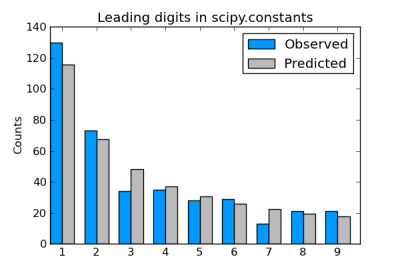
Sets of physical constants often satisfy Benford’s law, as I showed here for the constants defined in SciPy.

Incidentally, factorials satisfy Benford’s law exactly in the limit.

Weibull distributions

The Weibull distribution is a generalization of the exponential distribution. It’s a convenient distribution for survival analysis because it can have decreasing, constant, or increasing hazard, depending on whether the value of a shape parameter γ is less than, equal to, or greater than 1 respectively. The special case of constant hazard, shape γ = 1, corresponds to the exponential distribution.

Weibull and Benford

If the shape parameter of a Weibull distributions is “not too large” then samples from that distribution approximately follow Benford’s law (source). We’ll explore this statement with a little Python code.

SciPy doesn’t contain a Weibull distribution per se, but it does have support for a generalization of the Weibull known as the exponential Weibull. The latter has two shape parameters. We set the first of these to 1 to get the ordinary Weibull distribution.

      from math import log10, floor
      from scipy.stats import exponweib

      def leading_digit(x):
          y = log10(x) % 1
          return int(floor(10**y))

      def weibull_stats(gamma):

          distribution = exponweib(1, gamma)
          N = 10000
          samples = distribution.rvs(N)
          counts = [0]*10
          for s in samples:
              counts[ leading_digit(s) ] += 1

      print (counts)

Here’s how the leading digit distribution of a simulation of 10,000 samples from an exponential (Weibull with γ = 1) compares to the distribution predicted by Benford’s law.

      |---------------+----------+-----------|
      | Leading digit | Observed | Predicted |
      |---------------+----------+-----------|
      |             1 |     3286 |      3010 |
      |             2 |     1792 |      1761 |
      |             3 |     1158 |      1249 |
      |             4 |      851 |       969 |
      |             5 |      754 |       792 |
      |             6 |      624 |       669 |
      |             7 |      534 |       580 |
      |             8 |      508 |       511 |
      |             9 |      493 |       458 |
      |---------------+----------+-----------|

Looks like a fairly good fit. How could we quantify the fit so we can compare how the fit varies with the shape parameter? The most common approach is to use the chi-square goodness of fit test.

      def chisq_stat(O, E):
          return sum( (o - e)**2/e for (o, e) in zip(O, E) )

Here “O” stands for “observed” and “E” stands for “expected.” The observed counts are the counts we actually saw. The expected values are the values Benford’s law would predict:

      expected = [N*log10((i+1)/i) for i in range(1, 10)] 

Note that we don’t want to pass counts to chisq_stat but counts[1:] instead. This is because counts starts with 0 index, but leading digits can’t be 0 for positive samples.

Here are the chi square goodness of fit statistics for a few values of γ. (Smaller is better.)

      |-------+------------|
      | Shape | Chi-square |
      |-------+------------|
      |   0.1 |      1.415 |
      |   0.5 |      9.078 |
      |   1.0 |     69.776 |
      |   1.5 |    769.216 |
      |   2.0 |   1873.242 |
      |-------+------------|

This suggests that samples from a Weibull follow Benford’s law fairly well for shape γ < 1, i.e. for the case of decreasing hazard.

Related posts

Recreating the Vertigo poster

In his new book The Perfect Shape, Øyvind Hammer shows how to create a graph something like the poster for Alfred Hitchcock’s movie Vertigo.

Poster from Hitchcock's Vertigo

Hammer’s code uses a statistical language called Past that I’d never heard of. Here’s my interpretation of his code using Python.

      import matplotlib.pyplot as plt
      from numpy import arange, sin, cos, exp
      
      i  = arange(5000)
      x1 = 1.0*cos(i/10.0)*exp(-i/2500.0)
      y1 = 1.4*sin(i/10.0)*exp(-i/2500.0)
      d  = 450.0
      vx = cos(i/d)*x1 - sin(i/d)*y1
      vy = sin(i/d)*x1 + cos(i/d)*y1
      
      plt.plot(vx, vy, "k")
      
      h = max(vy) - min(vy)
      w = max(vx) - min(vx)
      plt.axes().set_aspect(w/h)
      plt.show()

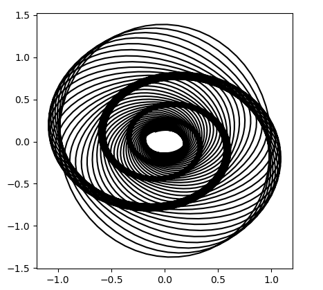
This code produces what’s called a harmonograph, related to the motion of a pendulum free to move in x and y directions:

Harmonograph

It’s not exactly the same as the movie poster, but it’s definitely similar. If you find a way to modify the code to make it closer to the poster, leave a comment below.

Approximate inverse of the gamma function

The other day I ran across a blog post by Brian Hayes that linked to an article by David Cantrell on how to compute the inverse of the gamma function. Cantrell gives an approximation in terms of the Lambert W function.

In this post we’ll write a little Python code to kick the tires on Cantrell’s approximation. The post also illustrates how to do some common tasks using SciPy and matplotlib.

Here are the imports we’ll need.

      import matplotlib.pyplot as plt
      from scipy import pi, e, sqrt, log, linspace
      from scipy.special import lambertw, gamma, psi
      from scipy.optimize import root

First of all, the gamma function has a local minimum k somewhere between 1 and 2, and so it only makes sense to speak of its inverse to the left or right of this point. Gamma is strictly increasing for real values larger than k.

To find k we look for where the derivative of gamma is zero. It’s more common to work with the derivative of the logarithm of the gamma function than the derivative of the gamma function itself. That works just as well because gamma has a minimum where its log has a minimum. The derivative of the log of the gamma function is called ψ and is implemented in SciPy as scipy.special.psi. We use the function scipy.optimize.root to find where ψ is zero.

The root function returns more information than just the root we’re after. The root(s) are returned in the arrayx, and in our case there’s only one root, so we take the first element of the array:

      k = root(psi, 1.46).x[0]

Now here is Cantrell’s algorithm:

      c = sqrt(2*pi)/e - gamma(k)
      
      def L(x):
          return log((x+c)/sqrt(2*pi))
      
      def W(x):
          return lambertw(x)
      
      def AIG(x):
          return L(x) / W( L(x) / e) + 0.5

Cantrell uses AIG for Approximate Inverse Gamma.

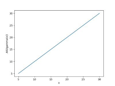
How well goes this algorithm work? For starters, we’ll see how well it does when we do a round trip, following the exact gamma with the approximate inverse.

      x = linspace(5, 30, 100)
      plt.plot(x, AIG(gamma(x)))
      plt.show()

This produces the following plot:

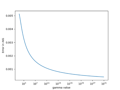
We get a straight line, as we should, so next we do a more demanding test. We’ll look at the absolute error in the approximate inverse. We’ll use a log scale on the x-axis since gamma values get large quickly.

      y = gamma(x)
      plt.plot(y, x- AIG(y))
      plt.xscale("log")
      plt.show()

This shows the approximation error is small, and gets smaller as its argument increases.

Cantrell’s algorithm is based on an asymptotic approximation, so it’s not surprising that it improves for large arguments.

More gamma function posts

Fat-tailed random matrices

Suppose you fill the components of a matrix with random values. How are the eigenvalues distributed?

We limit our attention to large, symmetric matrices. We fill the entries of the matrix on the diagonal and above the diagonal with random elements, then fill in the elements below the diagonal by symmetry.

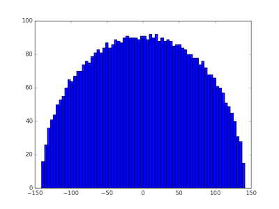
If we choose our random values from a thin-tailed distribution, then Wigner’s semicircle law tells us what to expect from our distribution. If our matrices are large enough, then we expect the probability density of eigenvalues to be semicircular. To illustrate this, we’ll fill a matrix with samples from a standard normal distribution and compute its eigenvalues with the following Python code.

      import numpy as np
      import matplotlib.pyplot as plt

      N = 5000
      A = np.random.normal(0, 1, (N, N))    
      B = (A + A.T)/np.sqrt(2)
      eigenvalues = np.linalg.eigvalsh(B) 
      print(max(eigenvalues), min(eigenvalues))

      plt.hist(eigenvalues, bins=70)
      plt.show()

We first create an N by N non-symmetric matrix, then make it symmetric by adding it to its transpose. (That’s easier than only creating the upper-triangular elements.) We divide by the square root of 2 to return the variance of each component to its original value, in this case 1. The eigenvalues in this particular experiment ran from −141.095 to 141.257 and their histogram shows the expected semi-circular shape.

eigenvalue distribution with normally distributed matrix entries

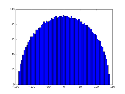
Wigner’s semicircle law does not require the samples to come from a normal distribution. Any distribution with finite variance will do. We illustrate this by replacing the normal distribution with a Laplace distribution with the same variance and rerunning the code. That is, we change the definition of the matrix A to

      A = np.random.laplace(0, np.sqrt(0.5), (N, N))

and get very similar results. The eigenvalues ran from −140.886 to 141.514 and again we see a semicircular distribution.

eigenvalue distribution for matrix with entries drawn from Laplace distribution

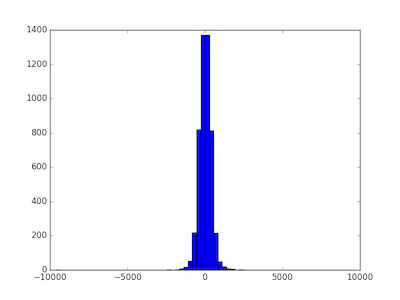
But what happens when we draw samples from a heavy-tailed distribution, i.e. one without finite variance? We’ll use a Student-t distribution with ν = 1.8 degrees of freedom. When ν > 2 the t-distribution has variance ν/(ν − 2), but for smaller values of ν it has no finite variance. We change the definition of the matrix A to the following:

      A = np.random.standard_t(1.8, (N, N))

and now the distribution is quite different.

eigenvalue distribution for matrix with entries drawn from Student t distribution with 1.8 degrees of freedom

In this case the minimum eigenvalue was −9631.558 and the largest was 9633.853. When the matrix components are selected from a heavy-tailed distribution, the eigenvalues also have a heavier-tailed distribution. In this case, nearly all the eigenvalues are between -1000 and 1000, but the largest and smallest were 10 times larger. The eigenvalues are more variable, and their distribution looks more like a normal distribution and less like a semicircle.

The distributions for all thin-tailed symmetric matrices are the same. They have a universal property. But each heavy-tailed distribution gives rise to a different distribution on eigenvalues. With apologies to Tolstoy, thin-tailed matrices are all alike; every thick-tailed matrix is thick-tailed in its own way.

Update: As the first comment below rightfully points out, the diagonal entries should be divided by 2, not sqrt(2). Each of the off-diagonal elements of A + AT are the sum of two independent random variables, but the diagonal elements are twice what they were in A. To put it another way, the diagonal elements are the sum of perfectly correlated random variables, not independent random variables.

I reran the simulations with the corrected code and it made no noticeable difference, either to the plots or to the range of the eigenvalues.

Rapidly mixing random walks on graphs

Random walks mix faster on some graphs than on others. Rapid mixing is one of the ways to characterize expander graphs.

By rapid mixing we mean that a random walk approaches its limiting (stationary) probability distribution quickly relative to random walks on other graphs.

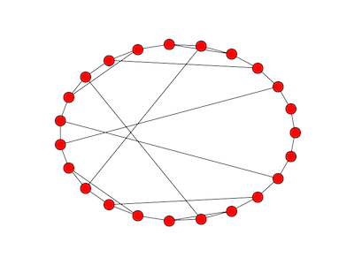
Here’s a graph that supports rapid mixing. Pick a prime p and label nodes 0, 1, 2, 3, …, p − 1. Create a circular graph by connecting each node k to (k + 1) mod p.  Then add an edge between each non-zero k to its multiplicative inverse mod p. If an element is its own inverse, add a loop connecting the node to itself. For the purpose of this construction, consider 0 to be its own inverse. This construction comes from [1].

Here’s what the graph looks like with p = 23.

Cayley graph of order 23

This graph doesn’t show the three loops from a node to itself, nodes 1, 0, and 22.

At each node in the random walk, we choose an edge uniformly and follow it. The stationary distribution for a random walk on this graph is uniform. That is, in the long run, you’re equally likely to be at any particular node.

If we pick an arbitrary starting node, 13, and take 30 steps of the random walk, the simulated probability distribution is nearly flat.

By contrast, we take a variation on the random walk above. From each node, we move left, right, or stay in place with equal probability. This walk is not as well mixed after 100 steps as the original walk is after only 30 steps.

You can tell from the graph that the walk started around 13. In the previous graph, evidence of the starting point had vanished.

The code below was used to produce these graphs.

To investigate how quickly a walk on this graph converges to its limiting distribution, we could run code like the following.

    from random import random
    import numpy as np
    import matplotlib.pyplot as plt
    m = 23

    # Multiplicative inverses mod 23
    inverse = [0, 1, 12, 8, 6, 14, 4, 10, 3, 18, 7, 21, 2, 16, 5, 20, 13, 19, 9, 17, 15, 11, 22]

    # Verify that the inverses are correct
    assert(len(inverse) == m)
    for i in range(1, m):
        assert (i*inverse[i] % 23 == 1)

    # Simulation
    num_reps = 100000
    num_steps = 30

    def take_cayley_step(loc):
        u = random() * 3
        if u < 1: # move left
            newloc = (loc + m - 1) % m
        elif u < 2: # move right
            newloc = (loc + 1) % m
        else:
            newloc = inverse[loc] # or newloc = loc
        return newloc

    stats = [0]*m
    for i in range(num_reps):
        loc = 13 # arbitrary fixed starting point
        for j in range(num_steps):
            loc = take_cayley_step(loc)
        stats[loc] += 1

    normed = np.array(stats)/num_reps
    plt.plot(normed)
    plt.xlim(1, m)
    plt.ylim(0,2/m)
    plt.show()

Related posts

* * *

[1] Shlomo Hoory, Nathan Linial, Avi Wigderson. “Expander graphs and their applications.” Bulletin of the American Mathematical Society, Volume 43, Number 4, October 2006, pages 439–561.

Random squares

In geometry, you’d say that if a square has side x, then it has area x2.

In calculus, you’d say more. First you’d say that if a square has side near x, then it has area near x2. That is, area is a continuous function of the length of a side. As the length of the side changes, there’s never an abrupt jump in area. Next you could be more specific and say that a small change Δx to a side of length x corresponds to approximately a change of 2x Δx in the area.

In probability, you ask what is the area of a square like if you pick the length of its side at random. If you pick the length of the side from a distribution with mean μ, does the distribution of the area have mean μ2? No, but if the probability distribution on side length is tightly concentrated around μ, then the distribution on area will be concentrated near μ2. And you can approximate just how near the area is to μ2 using the delta method, analogous to the calculus discussion above.

If the distribution on side lengths is not particularly concentrated, finding the distribution on the area is more interesting. It will depend on the specific distribution on side length, and the mean area might not be particularly close to the square of the mean side length. The function to compute area is trivial, and yet the question of what happens when you stick a random variable into that function is not trivial. Random variables behave as you might expect when you stick them into linear functions, but offer surprises when you stick them into nonlinear functions.

Suppose you pick the length of the side of a square uniformly from the interval [0, 1]. Then the average side is 1/2, and so you might expect the average area to be 1/4. But the expected area is actually 1/3. You could see this a couple ways, analytically and empirically.

First an analytical derivation. If X has a uniform [0, 1] distribution and Z = X2, then the CDF of Z is

Prob(Z ≤ z) = Prob(X ≤ √z) = √ z.

and so the PDF for Z, the derivative of the CDF, is −1/2√z. From there you can compute the expected value by integrating z times the PDF.

You could check your calculations by seeing whether simulation gives you similar results. Here’s a little Python code to do that.

      from random import random
      N = 1000000
      print( sum( random()**2 for _ in range(N) )/N )

When I run this, I get 0.33386, close to 1/3.

Now lets look at an exponential distribution on side length with mean 1. Then a calculation similar to the one above shows that the expected value of the product is 2. You can also check this with simulation. This time we’ll be a little fancier and let SciPy generate our random values for us.

      print( sum(expon.rvs(size=N)**2)/N )

When I ran this, I got 1.99934, close to the expected value of 2.

You’ll notice that in both examples, the expected value of the area is more than the square of the expected value of the side. This is not a coincidence but consequence of Jensen’s inequality. Squaring is a convex function, so the expected value of the square is larger than the square of the expected value for any random variable.

Distribution of numbers in Pascal’s triangle

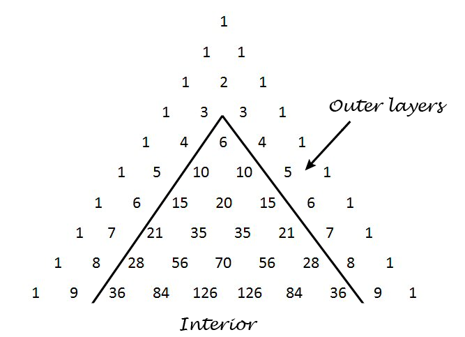
This post explores a sentence from the book Single Digits:

Any number in Pascal’s triangle that is not in the outer two layers will appear at least three times, usually four.

Pascal’s triangle contains the binomial coefficients C(n, r) where n ranges over non-negative numbers and r ranges from 0 to n. The outer layers are the elements with r equal to 0, 1, n-1, and n.

Pascal's triangle

We’ll write some Python code to explore how often the numbers up to 1,000,000 appear. How many rows of Pascal’s triangle should we compute? The smallest number on row n is C(n, 2). Now 1,000,000 is between C(1414, 2) and C(1415, 2) so we need row 1414. This means we need N = 1415 below because the row numbers start with 0.

I’d like to use a NumPy array for storing Pascal’s triangle. In the process of writing this code I realized that a NumPy array with dtype int doesn’t contain Python’s arbitrary-sized integers. This makes sense because NumPy is designed for efficient computation, and using a NumPy array to contain huge integers is unnatural. But I’d like to do it anyway, and the way to make it happen is to set dtype to object.

    import numpy as np
    from collections import Counter
    
    N = 1415 # Number of rows of Pascal's triangle to compute
    
    Pascal = np.zeros((N, N), dtype=object)
    Pascal[0, 0] = 1
    Pascal[1,0] = Pascal[1,1] = 1
    
    for n in range(2, N):
        for r in range(0, n+1):
            Pascal[n, r] = Pascal[n-1, r-1] + Pascal[n-1, r]
    
    c = Counter()
    for n in range(4, N):
        for r in range(2, n-1):
            p = Pascal[n, r]
            if p <= 1000000:
                c[p] += 1

When we run this code, we find that our counter contains 1732 elements. That is, of the numbers up to one million, only 1732 of them appear inside Pascal’s triangle when we disallow the outer two layers. (The second layer contains consecutive integers, so every positive integer appears in Pascal’s triangle. But most integers only appear in the second layer.)

When Single Digits speaks of “Any number in Pascal’s triangle that is not in the outer two layers” this cannot refer to numbers that are not in the outer two layers because every natural number appears in the outer two layers. Also, when it says the number “will appear at least three times, usually four” it is referring to the entire triangle, i.e. including the outer two layers. So another way to state the sentence quoted above is as follows.

Define the interior of Pascal’s triangle to be the triangle excluding the outer two layers. Every number n in the interior of Pascal’s triangle appears twice more outside of the interior, namely as C(n, 1) and C(n, n-1). Most often n appears at least twice in the interior as well.

This means that any number you find in the interior of Pascal’s triangle, interior meaning not in the two outer layers, will appear at least three times in the full triangle, usually more.

Here are the statistics from our code above regarding just the interior of Pascal’s triangle.

  • One number, 3003, appears six times.
  • Six numbers appear four times: 120, 210, 1540, 7140, 11628, and 24310.
  • Ten numbers appear only once: 6, 20, 70, 252, 924, 3432, 12870,  48620, 184756, and 705432.
  • The large majority of numbers, 1715 out of 1732, appear twice.